Explicit and implicit error correction methods の基礎概念 (数値解析における理論・手法・応用)

Explicit

and

implicit

error

correction

methods

の基礎概念

Basic

concept

of

explicit

and

implicit

error

correction

methods

岩下武史 (京都大学), 美舩健 (京都大学), 島崎眞昭 (福井工業大学)

Takeshi Iwashita (Kyoto University), Takeshi Mifune (Kyoto University), and Masaaki

Shi-masaki (Fukui University ofTechnology)

1

Introduction

This

paper

introduces the explicit and implicit

error

correction methods recently proposed by

the

authors [1]. First,

we

focus

on a

similarity

between

Hiptmair’s hybrid smoother [2] and

a

(2-level) multigrid method [3]. Both methods use a coefficient matrix that is different to the

originalonein theerrorcorrection process. While thehybridsmootherusesthediscrete gradient

operator matrix, the multigrid method introduces coefficient matrices constructed

on

the

coarse

grids. We define a

new

class of such

error

correction techniques in iterative solvers, which

we

call the Explicit $emr$ correction $(EEC)$ method. _{Moreover, corresponding to this explicit}

error

correction method,

we

have proposed the Implicit $emr$ correction $(IEC)$ method [1]. In

Section

2,

we

introduce the detail of both these methods.

Next,

we

showanexampleof the EEC andIECmethods inacontext of

an

electromagnetic field

analysis. In

a

finite element electromagnetic field analysis, it is necessary to solve a large linear

system ofequations. Generally,

a

linear iterativesolver such

as

theICCG (Incomplete Cholesky

Conjugate Gradient) method is used for this purpose [4]. It is well-known that the A-phi

formulation

gives

a

superior

convergence

rate to the

A-formulation

in the

iterative

solver [5, 6].

While _{several research papers have investigated the advantage of the A-phi method [7, 8], we}

here provide another interpretation of its effectiveness. It is shown that the A-phi method

(formulation)

can

be

seen as

an IEC method corresponding to Hiptmair’s hybrid smoother.

The authors have, therefore, suggested that the A-phi method has a similar effect to that of

the hybrid smoother for the

error

that corresponds to the kemel of the discrete curl operator

Ker(curl) [1]. Whereasthe hybrid smoother corrects these

errors

explicitly, the A-phi method

introduces unknown variables for the electric scalar potential. Numerical results show that

the A-phi method reduces the

error

belonging to Ker(curl) in the conductive region, which is

explicitly corrected in the hybrid smoother, more efficiently than the A-method.

Next, it is shown that the IEC method can improve the condition ofa coefficient matrix. We

introduce

our

new

multigrid type iterative method, namely the Implicit correction multigrid

method [9], which is

an

IEC method corresponding to

a

conventional multigrid method.

Nu-merical results of a 2-D finite difference analysis show that the implicit correction multigrid

method achieves

a

convergence rate independent of the grid-size, which is the most

impor-tant function of the multigrid method. Thus, the IEC method

can

improve the condition of

a

2

Explicit and

Implicit

Error

Correction

Methods

In this paper,

we

deal with

a

following linear sysytem ofequations:

$Ax=b$, (1)

where $A$ is

an

_{$n\cross n$} matrix, and

$x$ and $b$

are

n-dimensional vectors. When

a

linear system

(1) is solved by

an

iterative solver, the

error

_{correction method is often used. Let the current}

approximation for$x$be$\overline{x}$

.

The explicit

error

correction (EEC)methodisdefinedbythefollowing

two steps. The first step is to determine

error

quantity $\overline{y}$ using the following linear system:

$Cy=d(\tilde{x})$

.

(2)

When the dimension of$y$ is denoted by $m$, the coefficient matrix $C$ is

an

_{$m\cross m$} matrix. The

m-dimensional vector $d$ is given by a function of the current approximation $\tilde{x}$. In general, the

dimension $m$ is sufficiently smaller than $n$

.

Applying

an

iterative method such

as a

relaxation

method

or

a

direct solver to (2),

we

get an mdimensional vector $\tilde{y}$, which is

an

approximation

of$y$

or

exactly $y$

.

The second step is, then, given by the update ofthe approximation $\tilde{x}$:

$\tilde{x}^{new}arrow\tilde{x}+B\overline{y}$, (3)

where matrix $B$ is an _{$n\cross m$} matrix.

We here proposethe implicit

error

correction (IEC) method, inwhichthe original linear system

(1) and the (reduced dimensional) linear system for error correction (2) are combined. The

implicit

error

correction method is derived

as

follows. First, while

we

pay attention to (3),

the solution vector $x$ in (1) is replaced by $\hat{x}+B\hat{y}$, where $\hat{x}$ and

$\hat{y}$

are

n-dimensional and

m-dimensional vectors, respectively. This means that the solution vector is described by $\hat{x}+B\hat{y}$

.

Consequently,

we

obtain

$A\hat{x}+AB\hat{y}=b$ ₍₄₎

insteadof(1). Next,

we

consider the linear system for determining the

error

correction quantity

(2). In most explicit

error

correction type methods, the linear system (2) Is given by the

restricted residual equation of (1). In this case, $d$ is written

as

a matrix-vector product _$Dr$,

where $D$ is

an

_{$m\cross n$} matrix and _{$r=b-A\tilde{x}$ is the residual vector. Then, in}

the IEC method,

we

replace $d(\tilde{x})$ in (2) by _{$D(b-A\tilde{x})$}. Accordingly, we get

$DA\tilde{x}+Cy=Db$

.

₍₅₎

By rewriting vectors $\tilde{x}$ and

$y$ by $\hat{x}$ and

$\hat{y}$, respectively,

we

finally obtain the matrix form of the

IEC method

as

follows:

$(\begin{array}{ll}A ABDA C\end{array})(\begin{array}{l}\hat{x}\hat{y}\end{array})=(\begin{array}{l}bDb\end{array})$

.

(6)

In the proposed method, the linear system ofequations (6) instead of (1) is solved by

a

(pre.

conditioned) iterative method. The solutionofthe original linear system (1) is givenby $\hat{x}+B\hat{y}$

.

It is expected that the iterative solution process produces the effect of the error correction

implicitly. In other words, the linear system derived from the IEC method (6) is expected to

3

Relationship

Between

A-phi

Method and Hybrid

Smoother

In this paper, we deal with a quasi-static electromagnetic fieldproblem. It is assumed that the

analyzed domain $\Omega$ is a simply connected domain. For simplicity, we do

not describe the effect

of the boundary in the following. The basic equation based

on

the

A-formulation

is given by

$\nabla\cross(\nu\nabla\cross\vec{A}_{m})+\sigma\frac{\partial\vec{A}_{m}}{\partial t}=\vec{J_{0}}$,

(7) where $\vec{A}_{m},$

$\nu,$ $\sigma,$

$t,\vec{J_{0}}$

are

the magnetic vector potential, the magnetic reluctivity, the electrical

conductivity, time, and the excitingcurrent, respectively. It is notedthat $\nabla\cdot\tilde{J_{0}}=0$ is satisfied.

The basic equation based

on

the A-phi formulation is given by

$\nabla\cross(\nu\nabla\cross A_{m}^{\vec{/}})+\sigma\frac{\partial(A_{m}^{\vec{\prime}}+\nabla\phi)}{\partial t}=\vec{J_{0}}$,

(8)

$\nabla\cdot(\sigma\frac{\partial(A_{m}^{\vec{/}}+\nabla\phi)}{\partial t})=0$,

(9)

where $A_{m}^{\vec{\prime}}$ is also the magnetic vector potential and $\phi$ is the electric scalar potential.

When

a

finiteelement discretizationwith edge elements anda backward time differencemethod

are

applied to (7), the resulting linear system of equations is given by

$K_{A}x_{A}=(C_{u}^{T}M_{\nu}C_{u}+ \frac{M_{\sigma}}{\Delta t})x_{A}=b_{A}$, (10)

where $\Delta t$is the length ofthe timestep,

$x_{A}$ isthe unknown vector that represents the magnetic

vector potential tobecalculated, and the right-hand side$b_{A}$ isdetermined by thepreviousvalue

ofthe magnetic vector potentialand the exciting current. When the number of edges and faces

are

denoted by $e$ and $f$, respectively, the matrix $C_{u}$ is

an

$f\cross e$ matrix, which is given by the

discrete curl operator. The $f\cross f$ matrix $M_{\nu}$ and the $e\cross e$ matrix $M_{\sigma}$

are

given by

$[M_{\nu}]_{ij}= \int_{\Omega}\nu\vec{w}_{i}^{f}\cdot\vec{w}_{j}^{f}dV$, $[M_{\sigma}]_{ij}= \int_{\Omega}\sigma w_{i}^{\neg e}\cdot\vec{w}_{j}^{e}dV$, (11)

where $\vec{w}^{f}$ and $\vec{w}^{e}$

are a

face-element basis function and

an

edge-element basis function,

respec-tively.

In thispaper,

we

consider the

use

of Hiptmair’s hybrid smoother [2] in the A-method. Although

the hybrid smoother consists of a normal Gauss-Seidel sweep and

a

special

error

correction

process, the latter correction process is key to the method. Thus, we discuss only the

error

correction process in the following. When Hiptmair’s hybrid smoother is applied to (10), the

error

correction procedure can be written in the form ofan EEC method

as

follows:

$d(\overline{x}A)=G^{T}(b_{A}-K_{A}\tilde{x}_{A})$ ₍₁₃₎

in (2), and

$B=G$, ₍₁₄₎

where$\tilde{x}_{A}$ isthe current approximationfor

$x_{A}$ and $G$ is

a

discretegradient operatorthat satisfies $C_{u}G=0$

.

The matrix$C$is also written

as

$G^{T}K_{A}G$

.

From _{(6), (10), (12), (13), and (14) andthe} relationship between $C_{u}$ and $G$,

we

obtain the linear system ofthe

IEC

method corresponding

to the hybrid smoother

as

follows:

$(\begin{array}{ll}K_{A} K_{A}GG^{T}K_{A} G^{T}K_{A}G\end{array})(\begin{array}{l}\hat{x}_{A}\hat{y}_{A}\end{array})$

$=$ $(\Gamma^{1}\iota^{G^{T}M_{\sigma}}K_{A}$ $\tau_{t^{c^{M_{\sigma}G}}}^{1^{\Gamma^{1}t}\tau_{M_{\sigma}G}})(\begin{array}{l}x_{A}\hat{y}_{A}\end{array})=(\begin{array}{l}b_{A}G^{T}b_{A}\end{array})$

.

(15) The coefficientmatrix in (15) is identicalto the coefficient matrix arising from the finiteelement discretization of (8) and (9). Moreover, since the initial condition that $\hat{x}_{A}=x_{A}$ and $\hat{y}_{A}=0$ is

normally set at $t=0,$ $xA=\hat{x}_{A}+G\hat{y}_{A}$ is satisfied ineach time step. Consequently, the _right-hand

side of (15) is the

same

as the right-hand side derived from (8) and (9). Therefore, the linear

system of the IEC method that corresponds to the hybrid smoother (15) _{coincides with the}

linear system of equations _{derived from the A-phi method. Thus, the A-phi method}

_can

_be

regarded

as

the implicit version of the

error

correction of Hiptmair’s hybrid smoother.

4

Implicit

_Correction

_Multigrid

_Method

In this section,

we

introduce the implicit correction multigrid method [1, 9], in which the linear

systems of equations

on

all levels in

a

conventional multigrid method

are

combined and are

solved simultaneously using

a

_{(preconditioned) iterative method. We first introduce the 2-level}

implicit correction multigrid method. In a conventiona12-level multigrid method, the

coarse

grid correction for (1) is given in the form of the explicit

error

correction method

as

follows:

$C=A^{H}$_{, (16)}

$d(\overline{x})=I_{h}^{H}(b-A\tilde{x})$, ₍₁₇₎

and

$B=I_{H}^{h}$, ₍₁₈₎

where $A^{H}$ is the coefficient matrix

constructed

on

the

coarse

grid, and $I_{h}^{H}$ and $I_{H}^{h}$

are

the

restriction and prolongation operators, _{respectively. From} (6), (16), (17), and (18), the linear

system _{of the} (2-level) implicit _{correction multigrid method that} corresponds to the

coarse

grid

correction is given by

where $x^{H}$ is

an

unknown vector with the dimension of the

coarse

grid.

The linear system for the multi-level implicit correction multigrid method is derived from the

recursive application of the 2-level implicit correction multigrid method to the original linear

system (1). Here,

we

denote the linear system arising from the proposed method, for $0$ to $k$

levels, by

$T^{k}x_{t}^{k}=b_{t}^{k}$. (20)

When

we

solve (20) by

means

of the 2-level implicit correction multigrid method, the resulting

linear system is given by

$(I_{k}^{k+1}T^{k}T^{k}$ $T^{k}I_{k+1}^{k}A^{k+1})(x^{k+1}x_{t}^{k})=(\begin{array}{l}b_{t}^{k}I_{k}^{k+l}b_{t}^{k}\end{array})$ , (21)

where $A^{k+1}$ and $x^{k+1}$ are the coefficient matrix and the unknown vector on _{the $k+$llevel,}

respectively, and $I_{k}^{k+1}$ and $I_{k+1}^{k}$

are

the restriction and prolongationoperatorsbetween the k-th

and $(k+1)$-th levels, respectively. Applying (21) to (1) recursively,

we

finally obtain _{the linear}

system for the l-level implicit correction multigrid method

as

follows:

$(\begin{array}{lll}S^{0,0} \cdots S^{0,l}| \ddots |S^{l,0} \cdots S^{l,l}\end{array})(\begin{array}{l}x^{0}|x^{l}\end{array})=(\begin{array}{l}f^{0}|f^{l}\end{array})$ , (22)

where

$S^{\alpha,\alpha}=A^{\alpha}$, (23)

$S^{\alpha,\beta}=A^{\alpha}I_{\alpha+1}^{\alpha}I_{\alpha+2}^{\alpha+1}\cdots I_{\beta}^{\beta-1}(\alpha<\beta)$, (24)

$S^{\alpha,\beta}=I_{\alpha-1}^{\alpha}I_{\alpha-2}^{\alpha-1}\cdots I_{\beta}^{\beta+1}A^{\beta}(\alpha>\beta)$, (25)

$f^{\alpha}=I_{\alpha-1}^{\alpha}I_{\alpha-2}^{\alpha-1}\cdots I_{0}^{1}b$, (26)

$A^{0}=A$_{, and} $f^{0}=b$

.

_{In the proposed method, the linear system (22) is solved using}

_a

preconditioned iterative method. The solution vector of the original linear system (1) is given

by $x=x^{0}+ \sum_{k=1}^{l}\{(\prod_{p=1}^{k}I_{p}^{p-1})x^{k}\}$

.

5

Numerical

Results

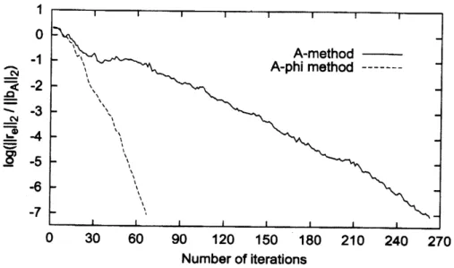
5.1 Effect of the A-phi

Method

In this subsection, we examine the effect of the

error

correction in the A-phi method. The test

problem is the TEAM (Testing Electromagnetic Analysis Method) workshop problem 10 [10].

The test model is discretized by using tetrahedrafinite elements (Whitney elements), with the

number of elements equal to 5968, and $\Delta t$ set to _$10^{-3}(s)$

.

The linear system in the first time

Number ofiterations

Figure 1: Comparison of

convergence

between

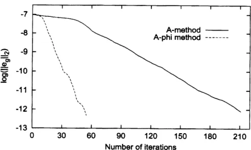
_{A-method and A-phi method}

$e_{g}$ of the kemel ofthe

discrete

curl operator $Ker(cur1)$ in the conductive region of

the model.

Whereas_{Hiptmair’s hybrid smoother corrects this}

_error

_{explicitly, Fig. 2indicates thatthe}

_error

$e_{g}$ can be efficiently removed in the A-phi method. Moreover, while we

calculate the 2-norm

ratio of$e_{9}$ with respect to thetotal

error

inthe conductive region for the A-method, the ratio is

higher than

0.9

in mostof iterations. Thus, the$Ker(cur1)$

error

causes

_{the slowconvergence rate}

in the A-method. Accordingly, _{the A-phi method has the effect of (implicit)}

_error

_{correction of}

$e_{g}$

as

in the hybrid smoother, and therefore achieves the advantage in convergence.

5.2

Effect

of the Implicit

_Correction

Multigrid

Method

In this subsection,

we

examine the effect ofthe implicit correction multigrid method. The test

problem isgiven

as

a linear systemof equationsderived from

a

2-D Poissonequationdiscretized

by afive point difference method. Figures3 and 4 show acomparison ofconvergence behaviors,

where $iMG$”

implies _{the implicit correction multigrid method. When the CG (Conjugate}

Gradient)

or

ICCGmethod isapplied to the originallinearsystem, theconvergenceratedeclines

rapidly

as

the problem sizeincreases. On the other hand, when the linear system based

on

the

implicit correction multigrid method is solved using the CG method, the number of iterations

necessary

for

convergenoe

does not really depend on theproblem size. Since the proceduredoes

not include

any

conventional multigrid process, thisresult indicates that the implicit correction

multigrid method includes the

coarse

grid correction effect. Moreover, it is shown that the

condition number ofthe coefficient matrix of the implicit multigrid method is improved from

Number ofiterations

Figure 2: Convergence behavior of the

error

of the kemel of the discrete curl operator in the

conductive region

5.3

Effectiveness

of

Implicit

_{Error Correction Method}

Numerical results indicate that the IEC method improves a condition ofthe coefficient matrix

and attains a similar effect

as

the corresponding EEC method. We

now

consider the condition

under which the IEC method works well. In general, an EEC type method is introduced for

correction of the

error

$e_{s}$ that satisfies $Ae_{s}\simeq 0$

.

When $A$ is positive

or

semi-positive definite,

these

errors

belong to

a

space spanned by _{the eigenvectors having small eigenvalues, which}

_we

denote by $V_{s}$

.

Accordingly, it is expected that the IEC method

can

work well when the range

of $B$ gives

a

good approximation of$V_{s}$

.

In thiscase, $D$ and $C$

can

simply be set

as

$D=B^{T}$ _and

$C=B^{T}AB$ _{(Galerkin approximation), respectively, and then the enlarged linear system (6) is}

written

as

a

following singular linear systcm:

$(\begin{array}{ll}A ABB^{T}A B^{T}AB\end{array})(\begin{array}{l}x\hat{y}\end{array})=(\begin{array}{l}bB^{T}b\end{array})$. (27)

In

our

numerical tests, the implicit _{correction multigrid method shows good}

_convergence

per-formance under the above condition, even though the coefficient matrix on coarse levels can be

constmcted using other strategies. In [11],

we

have discussed the condition of the matrix$B$ for

making the IEC method work well.

6

Conclusion

This paper introduces proposed

an

implicit

error

correction method that corresponds to the

$\mathring{=}E$ コ $\underline{\frac{\varpi}{q\Phi^{)}}}$ $\geq\Phi$ $o\tilde{\frac{\varpi}{e\Phi}}$

Number

of

iterations

Figure 3: Comparison of

convergence

behaviors (15 $\cross 15$ grid)

correction in a multigrid method. It is shown that the A-phi method can be regarded as an

implicit

error

correction version of the hybridsmoother. Fhrthermore, numericaltestsshowthat

the A-phi methodhas a similar effect on the correction ofthe

error

ofthe kernelofthe discrete

curl operator

as

that of the _{hybrid smoother, which results in an advantage in convergence.}

Next, we introduce the implicit correction multigrid method by applying the implicit

error

correctionconcept _{to the multigrid method. It is shown that the proposed method achieves the}

convergence

rate independent of the problem size. This result confirms the strong relationship

between

theexplicit

error

correctionmethodand the implicit

error

correction methodandshows

the effectiveness of the proposed method.

References

[1] T. Iwashita, T Mifune and M. Shimasaki,

“Similarities

between implicit correction

multi-grid method and A-phi formulation _{in electromagnetic field analysis”, IEEE Thans. Magn.,}

vol.44, pp. 946-949, June, 2008.

[2] R. Hiptmair, “Multigrid method for Maxwell’s equations,” SIAM J. Numer. Anal., vol.36,

pp. 204-225, Dec. 1998.

[3] P. Wesseling, An introduction to multigrid methods, JohnWiley&Sons Ltd.,

1992.

Corrected

$CO\subseteq$ コ $\underline{\Phi\frac{\mathring}{\omega}}$ $\geq\omega$ $\check{\underline{\varpi}}$ $oe\omega$

Number

of

iterations

Figure 4: Comparison of

convergence

behaviors (127 $\cross 127$ grid)

[4] Y. Saad, Iterative Methods

_for

Sparse LinearSystems, Second ed., Philadelphia, PA: SIAM,

2003.

[5] K. Fujiwara, T. Nakata, and H. Ohashi, “Improvement of convergence characteristic of

ICCG method for the $A-\phi$ method using edge elements”, _{IEEE Trans. Magn., vol.32,}

pp. 804-807, May 1996.

[6] R.D. Edlinger and $0$

.

Biro, “A joint vector and scalar _potential formulation for driven

high frequencyproblemsusing hybrid edge and nodal finite element,” IEEE Tmns. Microw.

Theory Tech., vol.44, pp. 15-23, Jan. 1996.

[7] H. Igarashi and T. Honma, “_{On convergence}

ofICCG applied to finite element equation for

quasi-static _{fields,” IEEE Trons. Magn.,} vol.38, pp. 565-568, Mar. 2002.

[8] B. Weiss and O. Biro, “On the convergence of transient eddy-current problems,” IEEE

$\pi ans$

.

Magn., vol.40, pp. 957-960, Mar. 2004.

[9] T.Iwashita, T. Mifune, and M. Shimasaki,“

New multigrid method: basicconceptofimplicit

correction multigrid method,” IPSJ $\pi_{ans}$

.

Advanced Computing Systems, vol.48 _(ACS18),

pp. 1-10, May 2007 (In Japanese).

[10] T. Nakata, N. Takahashi, and K. lfujiwara,“_Summary

of the results for

benchmark

problem

[11] T. Mifune, S. Moriguchi, T. Iwashita, and M. Shimasaki, “Convergence

_Acceleration

_of

Iterative Solvers

_{for the Finite Element Analysis Using the Implicit and Explicit Error}