Analyzing Factors of Defect Correction Effort in a Multi-Vendor Information System Development

全文

(1)Analyzing Factors of Defect Correction Effort in a Multi-Vendor Information System Development Tomoko Matsumura Nara Institute of Science and Technology Keihanna Science City, 630-0192 Japan [email protected] Tel. +81-743-72-5318 Fax +81-743-72-5319. Akito Monden Nara Institute of Science and Technology, Keihanna Science City, 630-0192 Japan [email protected]. Shuji Morisaki Nara Institute of Science and Technology, Keihanna Science City, 630-0192 Japan [email protected]. Ken-ichi Matsumoto Nara Institute of Science and Technology Keihanna Science City, 630-0192 Japan [email protected].

(2) Analyzing Factors of Defect Correction Effort in a Multi-Vendor Information System Development ABSTRACT This paper describes an empirical study to reveal factors influencing defect correction effort in software development. In the study we collected various attributes (metrics) of defects found in a typical medium-scale, multi-vendor information system development project in Japan over a six-month period. We then statistically analyzed the relationship between the defects’ attributes and the correction effort. The analysis confirmed the well-known principle “defects are the more expensive the later they are detected” by revealing that defects detected in the “system test” were 4.88 times more expensive than those detected in the “coding/unit test”. Another principle “defects are more expensive the longer they survive in software” was also confirmed by revealing that defects, which survived two or more development phases, were 4.44 times more expensive than those detected immediately. We also identified other factors, such as defect repeatability, severity, and the cause of detection delay, that had a significant influence on the correction effort.. KEYWORDS Defect Classification, Statistical analysis, Failure Report, Testing.

(3) 1. INTRODUCTION Defects in software development, such as bugs, specification changes, and design changes, are a major cause of excessive cost (effort) and delivery slippage. Analysis methods have thus been proposed to investigate the number of defects found in each development phase and/or in each functionality and to reveal relations with the causes of the defects. One such example is orthogonal defect classification (ODC) [2][3][8]. This method identifies phases and processes that require improvement by classifying each defect into one of several categories based on failure reports and then by looking for variation in the numbers of defects of each type between phases and processes. Another example is defect causal analysis (DCA) [7][18][20]. This method collects detailed information on each defect and then hierarchically classifies causes of defects using cause-effect diagrams (fishbone diagrams)[15]. However, focusing on the number of defects is not sufficient for process improvement. In fact, there is a great deal of variance in the effort required to correct defects[16]. Even a single defect could cause a serious excess of correction effort or delay delivery. In this paper we analyze the relationship between the defect correction effort (person-hours) and the characteristics of defects, as well as the reasons why the defects were not detected upstream of development. Our goal is to avoid excessive correction cost (effort) and delivery slippage in software development. We collected attributes of the defects, such as the cause of a defect's introduction and the functionality of the module where the defect was found, as well as phases where the defect was introduced and detected. In the analysis, we statistically.

(4) detected the factors that influence the defect correction effort and then analyzed each factor in detail using box plots. Afterwards, we conducted further analysis on the relation between the phase where a defect is introduced and the phase where it is detected. This was done to validate the results of past research, such as the finding that the longer a defect survives in software the greater its correction effort becomes [11]. We also used information obtained from detailed descriptions of failure reports and interviews with the developers to interpret analysis results. This paper targets a multi-vendor development, which is the most typical type of information systems development in Japan today. Specifically, the target was an information system development project consisting of about 330K steps (SLOC) of C/C++ source code, carried out with the support of Japan's Ministry of Economy, Trade and Industry (METI). In this project, several core Japanese software companies carried out development, while the Nara Institute of Science and Technology's EASE Project 1 and Japan’s SEC 2 of the Information-Technology Promotion Agency collaboratively created a data-collection scheme and analyzed the obtained data. Development was carried out using a waterfall process. A user company defined requirements, and development companies each developed subsystems under the supervision of a project-management company. After each company conducted an intra-company unit test and integration test, an inter-company integration test was performed, followed by an inter-company. 1. EASE : Empirical Approach to Software Engineering. http://www.empirical.jp/project/index.html 2. SEC : Software Engineering Center http://sec.ipa.go.jp/index.php.

(5) system test. The difference between the analysis described in this paper and ODC/DCA is that here we used statistical analysis. Since defect counts are a per-project attribute, the statistical analysis that can be performed using this attribute within a single project is extremely limited. In contrast, defect correction effort is a per-defect attribute. This means that it can be used for statistical analysis even on a single project (given a large number of defects). A long-standing principle states that defects are more expensive the later they are removed[11]. Nevertheless, there exists almost no report that specifically identifies how much correction effort increases. The only such examples were done in the 1970s and early 80s by Boehm [5][6], Fagan[12], Daly[9] and Hiemann[13]. However, the systems in those examples are quite old; thus, the development/testing environment may be different from today's style of development. Also, the above papers did not describe relations to other defect characteristics, such as the cause of detection delay, defect repeatability and defect severity, etc. More detailed analysis on typical modern projects is required. In Section 2, we outline the data collected for use in analysis; Section 3 describes the analysis procedure. Section 4 presents the results of the analysis at each step; Section 5 describes related research; and in Section 6, we summarize our findings and discuss future work..

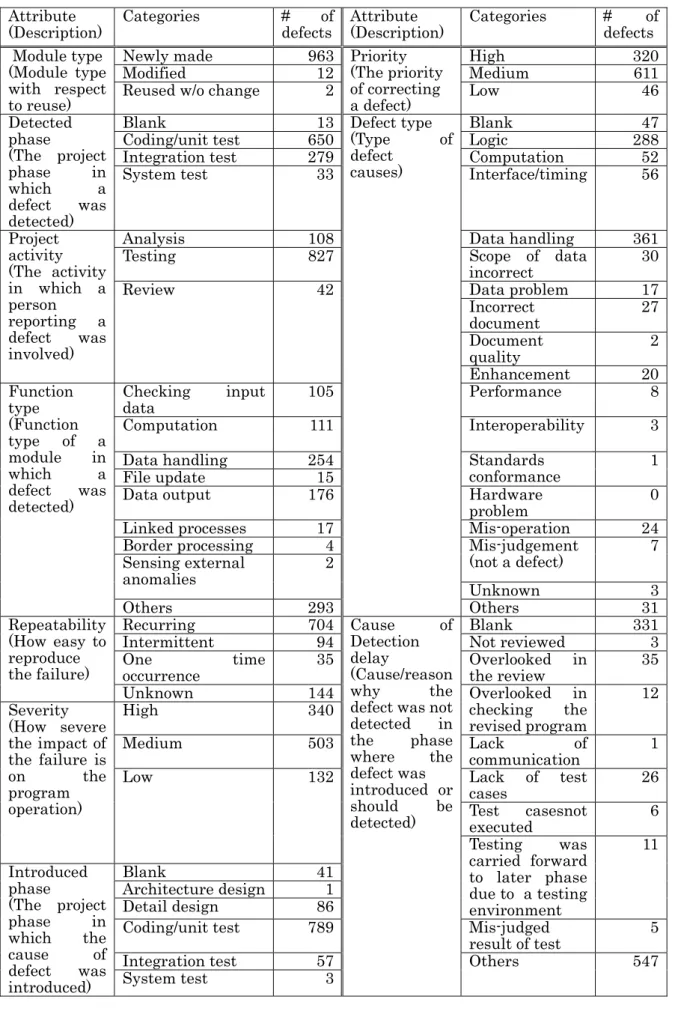
(6) Table 1 Attributes of Defects Attribute (Description) Module type (Module type with respect to reuse) Detected phase (The project phase in which a defect was detected) Project activity (The activity in which a person reporting a defect was involved) Function type (Function type of a module in which a defect was detected). Categories Newly made Modified Reused w/o change Blank Coding/unit test Integration test System test. 13 650 279 33. Analysis Testing. 108 827. Severity (How severe the impact of the failure is on the program operation). Introduced phase (The project phase in which the cause of defect was introduced). Attribute (Description) Priority (The priority of correcting a defect) Defect type (Type of defect causes). Categories High Medium Low. # of defects 320 611 46. Blank Logic Computation Interface/timing. 47 288 52 56. 361 30. Checking input data Computation. 105. Data handling Scope of data incorrect Data problem Incorrect document Document quality Enhancement Performance. 111. Interoperability. 3. Data handling File update Data output. 254 15 176. Standards conformance Hardware problem Mis-operation Mis-judgement (not a defect). 1. Review. 42. Linked processes Border processing Sensing external anomalies Repeatability (How easy to reproduce the failure). # of defects 963 12 2. Others Recurring Intermittent One occurrence Unknown High. time. 17 4 2 293 704 94 35 144 340. Medium. 503. Low. 132. Blank Architecture design Detail design Coding/unit test Integration test System test. 41 1 86 789 57 3. Cause of Detection delay (Cause/reason why the defect was not detected in the phase where the defect was introduced or should be detected). Unknown Others Blank Not reviewed Overlooked in the review Overlooked in checking the revised program Lack of communication Lack of test cases Test casesnot executed Testing was carried forward to later phase due to a testing environment Mis-judged result of test Others. 17 27 2 20 8. 0 24 7 3 31 331 3 35 12 1 26 6 11. 5 547.

(7) 2. COLLECTED DATA 2.1. Outline of Target Project We analyzed a project to develop a probe-information system carried out by members of the COSE3, with the support of METI. Six companies participated in the development: one company was tasked with project management, and the other five with development. Two of the five companies each conducted development at two different sites, with the result that the development was conducted at seven physically separated sites. From the start of the project, researchers from the EASE project and the SEC attended regular project meetings and were tasked with the creation of a data-collection scheme and data analysis. A facility was also set up where periodic meetings could be held with individual companies in order to report the analysis results to the developers. EASE and SEC researchers used these meetings to give feedback on analysis results and conduct interviews. The size of the developed system is approximately 330K steps (SLOC), and almost all of the source code was written in C/C++ language. The number of subsystems is 38 and the number of files including shell script, batch, etc. is approximately 1400.. 2.2. Defect Data and its Collection Process First, the defect attributes to be collected were determined through pre-project discussions, referring to failure reports actually used by the six participating. 3. COSE : COnsortium for Software Engineering.

(8) companies and the classification for software anomalies in IEEE Standard 1044-1993 [1]. If collected data is not accurate, complete, and consistent across the company, then incorrect results may be derived[13]. Thus, we discussed until all participants (project managers and quality assurance staffs) accepted and understood the definition of attributes. Nearly all of the companies ended up collecting attributes that were different from those they had traditionally collected. For example, two of the companies had never collected data on correction effort. Data were collected separately at each of the seven development sites. All but one of the sites introduced the GNATS4. The remaining site supported the scheme by customizing its standard in-house tool. The collected defect data were stored in a database at the SEC and analyzed using the Empirical Project Monitor (EPM) [21]. Data were collected from all seven sites; however, we excluded data from one site because data reliability was low, according to an interview with the developers, and the data had an unusual distribution. It was because each development site outsourced multiple organizations and in such complicated structure it often is difficult to manage developers’ activities[16][18]. The phases of development for which data were collected - that is, the phases where defects were detected - were those from coding/unit test to system test (in this project, coding and unit tests are considered parts of the same phase).. 4. GNATS : GNU Bug Tracking System http://www.gnu.org/software/gnats/.

(9) In this project, testing was carried out in the following stages: first, each site conducted the unit test and integration test internally; next, inter-company integration and system tests were conducted, integrating the products of all companies in an integrated environment. Defects introduced after the architecture-design phase were analyzed. For this project, errors and changes to the requirements specification were excluded from analysis, since they are managed by a different management procedure. Table 1 lists the collected defect attributes that were used for this paper. There. were also free-description reports, such as descriptions of the symptoms as well as details on a defect's cause, disposition, and confirmation, but these do not appear in the table because they were not used for the statistical analysis. For the purposes of statistical analysis, we refer to each attribute in Table 1 as a variable. This paper refers to defect correction effort as a dependent variable and to other variables as independent variables. Each possible value of a variable is called a category. For example, the variable severity has three possible categories: “high”, “medium”, and “low”.. 2.3. Summary of Collected Data Table 2 shows the statistics of defect correction effort. Available data, i.e. the number of defects whose correction efforts were recorded, amounted to 978. We excluded the remaining 39 from the analysis because they were either left blank or zero was input as the correction effort. While the mean correction effort was about 2 person-hours, the median value was just 1 person-hour, showing variance in the value distribution. The highest correction effort was 92 person-hours,.

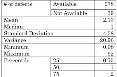
(10) corresponding to about 3.8 person-days.. 3. PROCEDURE OF DATA ANALYSIS We carried out the analysis using the following steps: (1) data preprocessing; (2) analysis of relationship between each variable and correction effort; and (3) analysis of relations between variables. We used information obtained from detailed descriptions of failure reports and interviews with the developers to interpret the analysis results. Each step is described in detail below. Table 2 Statistics of Defect Correction Effort (person-hours). # of defects. Available Not Available. Mean Median Standard Deviation Variance Minimum Maximum Percentile 25 50 75. 978 39 2.13 1 4.58 20.96 0.08 92 0.75 1 2. 3.1. Data Preprocessing Before conducting the analysis, we preprocessed the data as follows: . Handling of blank fields: “Blank” values in Table 1 were all treated as missing values.. . Adding detection delay: We created a new independent variable called. detection delay, indicating the delay between the phase where the defect was introduced (hereinafter called introduced-phase) and the phase where it was detected (hereinafter called detected-phase). This was a measure to confirm existing research showing that the longer a defect remains in a product, the.

(11) more expensive it is to remove[11].. 3.2. Analysis of Relation between Each Variable and Defect Correction Effort First, we analyzed the relations between the variables in Table 1 and correction effort, as well as the strength of these relations. We statistically analyzed the existence of a relation by using ANOVA(Analysis of Variance) and a t-test for the difference in the means of correction effort between defects belonging to a given category and those belonging to other categories for each independent variable. The criterion for significance was 1% (p < 0.01). Variables and categories having (significant) relations with correction effort were identified by using this t-test for all categories of all variables. The difference between the means of correction effort was used to determine the strength of a relation. Variables and categories with small differences (fewer than 1.0 person-hour) were excluded from the later analysis, even if they had significant deviation according to the t-test. In this paper, ANOVA and a t-test are thoroughly used for statistical analysis; they assume that a data set is normally distributed. However, an investigation of correction effort distribution by a normal P-P plot showed that the distribution is not normal. We then confirmed that correction effort did follow a normal distribution after logarithmic transformation, so ANOVA and t-tests were conducted after the transformation. Next, we analyzed in detail each phase-related variable (i.e. introduced-phase,. detected-phase, and detection delay). Box plots for each phase-related variable showed the impact that different phases had on correction effort..

(12) 3.3. Analysis of Relations between Variables In order to reveal the main factors affecting correction effort, it is necessary to analyze the relations. In this paper, we addressed only the relations between. introduced-phase and detected-phase due to space limitations. We categorized the defects by all combinations of introduced-phase and detected-phase, in the manner of ODC, and then analyzed statistically the differences in the means of correction effort among the combinations. Table 3 Categories that Showed Significance in t-test Independent Variables. Categories. # of Mean of Defects Defects Correction Effort. Detected phase Introduced phase Detection delay. Coding/unit test System test Detail design. 650 33 86. 1.70 8.29 3.89. 639 54 5 26 11. 1.70 7.54 4.80 5.84 7.55. Mis-judged result of test. 5. 4.00. Defect Type. Mis-judgement (not a defect). 7. 0.75. Repeatability. Other Intermittent One time occurrence. 31 94 35. 1.15 3.70 0.44. 132 42. 0.88 0.99. 978. 2.13. Cause detection delay. 0 Phase 2 Phases 3 Phases of Lack of test cases Testing was carried forward to later phase due to a testing environment. Severity Low Project Review Activity (Ex)All Defects. 4. RESULTS 4.1.. Relation between Each Variable and Defect Correction Effort. Firstly, based on ANOVA, we excluded the variable Module Type from our further.

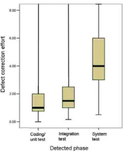
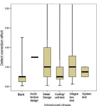
(13) analysis since it did not have significant relationship with defect correction effort (assuming 1% significance level). Table 3 lists the categories found to be significant by the t-test and having a significant difference of at least 1.0 person-hour from the mean of the other categories. The table columns show, from left to right, the independent variable, its category, number of defects in that category, and the mean correction effort. Below, we describe the results for each variable and/or category in the table in detail. [Detected Phase] When the Detected-phase was “coding/unit test,” the mean correction effort was small (1.7 person-hours), but when it was system test, it was large (8.29 person-hours). Figure 1 shows box plots of correction effort in each phase. The amount of effort required to correct a defect tended to increase when it was detected in a later phase. [Introduced phase] When the Introduced-phase was “detail design,” the mean correction effort was large (3.89 person-hours). Figure 2 shows box plots of correction effort in each phase.. Figure 1 Defect Correction Effort in Each Detected-Phase.

(14) Figure 2. Figure 3. Defect Correction Effort in Each Introduced-Phase. Defect Correction Effort in Each Detection Delay. [Detection delay and its causes] When the detection delay was zero (i.e.. Introduced-phase and Detected-phase were the same), the mean correction effort was low (1.7 person-hours). When the detection delay was two phases, this value increased to 7.54 person-hours, and at three phases it reached 4.80 person-hours (note, however, that only five defects had detection delays of three phases). Figure.

(15) 3 shows box plots of relations between detection delay and defect correction effort. The figure shows that although there is almost no difference in correction effort between delays of 0 and 1 phase, at two phases the value suddenly surges. Next, let us draw our attention to the causes of detection delay. Table 3 shows that the correction effort increases when the reason is “testing was carried forward to later phase due to a testing environment” (7.55 person-hours). This cause indicates cases where tests were required, but testing was delayed because a testing environment would not be available until the integration test or system test, thereby causing the detection of the defect to be delayed. The other causes, “lack of test cases” and “mis-judged result of test,” also increased the correction effort to 2 or 3 times more than the mean correction effort of all defects. [Defect type] Although there were not many such cases (only 7), the correction effort of defects caused by “mis-judgement” (defect reported but actually there was no defect) was low (0.75 person-hours). No significant relations were found between correction effort and other causes (of which there were many, including “logic,” “computation,” and “data handling” issues). Additionally, defects in the “others” category tended to require lower correction effort, but no breakdown of this category was done. [Repeatability] Correction effort was somewhat higher when repeatability was low (i.e. “intermittent”) (3.70 person-hours). We believe that this may be because defects with low reproducibility (where it was difficult to identify the location of the defect) took longer to debug. The correction effort of defects that never reoccurred (i.e. “one time occurrence”) was low, but the majority of them were defects detected during source code reviews, which do not execute the code, so.

(16) these defects never “occurred” in the program execution. [Severity/priority] Correction effort tended to be lower when the severity was low (0.88 person-hours). No difference was found between high and medium severities. We conjecture that this may be because the engineers selected “low” if they thought it was easy to find the location of the defect and how to correct it. Meanwhile, no relation was found between priority and defect correction effort. [Project activity] The correction effort was somewhat low when the detection process was (code) review (0.99 person-hours). We believe that this is because defects detected during reviews do not require a regression test. [Other variables] No relations were found between correction effort and the other two variables: module type and function type. We believe that no significant difference was found for module type because almost all defects were detected in newly developed areas (“newly made”), while nearly no defect was found in reused portions of the code. The system includes a large amount of modified and reused code, but there were few defects because the majority of the system was diverted from other highly reliable systems. More defects were detected in “data handling” of function type than any other. This was followed by “data output,” “computation,” and “checking input data,” in that order, but there was no significant difference in the mean correction effort per defect..

(17) Table 4 Results of t-test for Phase-related Variables Introduced phase. 4.2.. # of Mean of Defect p-value Defects Correction Effort. Detected phase=”Coding/unit test” Detail design 47 2.74 Coding/unit test 587 1.64. 0.307 0.911. Detected phase=”Integration test” Detail design 33 5.50 Coding/unit test 171 2.02 Integration Test 50 2.53. 0.000 0.016 0.160. Detected phase=”System test” Detail design 5 4.80 Coding/unit test 21 10.74 Integration test 6 3.67. 0.797 0.143 0.388. Relations between Variables. We calculated the mean defect correction effort for each combination of introduced. phases and detected phases and statistically compared them. For each detection phase, Table 4 shows, from left to right, categories of introduced phase, the number of defects in each introduced phase, the mean defect correction effort within the phase, and p-value of a t-test (between each target phase and others). Assuming the 1% significance level, there was no influence of introduction phase on defects detected in “coding/unit test” or “system test”(p>0.01). On the other hand, for defects detected in “integration test,” correction effort significantly increased when defects were introduced in “detail design” (5.5 person-hours). According to the results in the previous section 4.1, defects introduced in the earlier phase (i.e. “detail design”) required more effort for correction than those in later phases (3.89 person-hours). However, Table 4 shows that, even though defects were introduced in the design phase, they did not require so much effort when they were detected in the next phase, i.e. “coding/unit test”(2.74 person-hours), compared to when they were detected in the later phase, i.e..

(18) “integration test” (5.50 person-hours). On the other hand, even though defects were detected in the “integration test,” they required a small effort when they were introduced in the “coding/unit test”(2.02 person-hours). This confirms the results of the previous section 4.1, i.e. that a defect correction effort remarkably increased when detection delay involved two or more phases. Moreover, defects detected in the “system test” required much more effort than those detected upstream regardless of their introduced phase, according to Table 4. These results indicate the following: . “Design defects” are best detected by the unit test. If they are detected in the integration test phase, the correction effort will become much greater.. . “Coding Defects” are best detected in the code review or unit test phase; however, it would not seriously increase the correction effort even if they were detected in the integration test phase. However, correction effort surges when they are detected in the system test phase.. . Defects detected in the “system test” require much more effort than others regardless of their introduced phase.. Based on the interviews with the developers and the questionnaires they completed, we confirmed the following reasons for increased effort in system testing. . When finding a defect in the system test, the engineer had to locate the vendor or development site at which the cause of the defect was introduced. Sometimes this took much time because engineers were often unfamiliar with other vendors’ programs..

(19) . If the defect was related to more than one vendor's program, it took much time to modify the programs due to the need for excessive communication between vendors.. . The correction of a defect detected in the system test had to be confirmed by regression testing in an environment where all vendors' programs were integrated, as well as the database and hardware. The necessary preparation for regression testing of the system test required much more time than for intra-company unit/integration tests.. We also confirmed from the interviews that the above situations commonly occurred in many multi-vendor developments.. 5. RELATED WORKS Some studies have already analyzed the cost incurred by defects, e.g. Fagan's Study at IBM in 1976 [12], Daly's Study at GTE in 1977 [9], and Boehm's Study at TRW in 1974 [4]. Figure 4 shows a comparison of the these studies[6] with our study's results added. The horizontal axis shows the phases where a defect was detected, and the vertical axis shows the relative (logarithmic) effort of correcting defects, assuming the cost in the coding phase is 10..

(20) Figure 4 Boehm's Results[6] Vs. Japanese Multi-Vendor Project In the figure, the solid line shows the escalation in cost-to-fix versus phase at IBM[12], GTE[9],and TRW[4], and the dotted line shows the escalation for two smaller, less formal projects analyzed by Boehm[5]. As a result of the analysis, Boehm summarized: . The error (defect) is typically 100 times more expensive to correct in the maintenance phase on large projects than in the requirement phase[6].. . Although the effect on smaller projects is less pronounced, a 4:1 escalation in cost-to-fix between the requirement and the integration test is observed in Figure 4[5]..

(21) The results of our study, which are shown as rectangles in Figure 4, support these past results of the 1970s and 80s. In our study, defect correction effort in the system test is about four times larger on average than in the coding/unit test.. 6. SUMMARY This paper analyzed the factors that influence the defect correction effort and how these factors are related to each other, based on the defect data collected from a Japanese multi-vendor information system development project. Our findings include the following: . The well-known principle “defects are more expensive the later they are detected” was confirmed quantitatively. When defects were detected in the “coding/unit test” phase, the mean correction effort was small (1.7 person-hours), but when detected in the ”system test” phase, it became much larger (8.29 person-hours).. . Another principle, “defects are more expensive the longer they survive in software,” was also confirmed. When the detection delay (between defect introduced- and detected- phase) was zero, the mean correction effort was low (1.7 person-hours), but when the delay became two phases, it increased to 7.54 person-hours.. . Further analysis of defect introduced phase and detected phase revealed that defects detected in the “coding/unit test” have a low cost and those detected in the “system test” have a high cost regardless of their introduced phase. On the other hand, for defects detected in the “integration test,” correction effort significantly increased when they were introduced in “detail design” (5.5 person-hours). These results suggest that “design defects” are best detected by.

(22) the unit test and “coding defects” by the integration test phase. . Some causes of detection delay showed significant influences. The correction effort increased when the cause was “testing was carried forward to later phases due to the testing environment” (7.55 person-hours).. . Two other factors, severity and repeatability, also influenced the defect correction effort. The mean correction effort for low-severity defects was low (0.88 person-hours) and that for low-repeatability defects was high (3.70 person-hours).. These results would be useful for project managers to select more cost-effective, i.e. higher ROI (Return on Investment), actions in development. For example, to decrease the cost by detecting ”design defects” before the integration test, a project manager might assign different engineers to design and programming in order to check for design defects in the coding phase. On the other hand, if some test cases were difficult to execute upstream due to the testing environment, a manager would have to weigh the risks of carrying the test forward. Moreover, we found that in the multi-vendor development the result has strategic value as organizational level[22], and it shows importance of total quality management(TQM) with top management support from data collection to process improvement[9]. The major limitation of this paper is that we focused only on defects introduced at and after the design phase, and thus requirement defects were out of the scope of the current work. However, since requirement defects are usually more expensive to remove, we need to analyze the factors of their correction effort in future study..

(23) ACKNOWLEDGMENTS This work is supported by the Comprehensive Development of e-Society Foundation Software program of the Ministry of Education, Culture, Sports, Science and Technology. We thank the companies that belong to COSE (COnsortium for Software Engineering), researchers at SEC (Software Engineering Center) and the EASE Project for collaborating on the data collection and analysis..

(24) REFERENCES [1]. IEEE Standard 1044-1993 IEEE Standard Classification for Software Anomalies, 1993.. [2]. Bassin, K.A., Kratschmer, T., and Santhanam. P., ”Objectively evaluating software development,”, IEEE Software, 15(6), 1998, 66-74.. [3]. Bhandari, I., Halliday, M., Traver, E., Chaar, D.B.J., and Chillarege. R., “A case study of software process improvement during development,” IEEE Trans. on Software Engineering, 19(12), Dec, 1993, 1157-1170.. [4]. Boehm, B.W., “Software engineering,” IEEE Trans. on Computers, 25(12), 1976, 1226-1241.. [5]. Boehm, B.W., “Developing small-scale application software product: some experimental results,” In Proceedings of IFIP (International Federation for Information Processing) Congress, 1980, 321-326.. [6]. Boehm, B.W, Software Engineering Economics, Englewood Cliffs, NJ: Prentice-Hall, 1981.. [7]. Card, D., “Learning from our mistakes with defect causal analysis,” IEEE Software, 15(1), January/February 1998, 56-63.. [8]. Chillarege, R., Bhandari, I., Chaar, J., Halliday, M., Moebus, D., Ray, B., and Wong, M., “Orthogonal defect classification-a concept for in-process,” IEEE Trans. on Software Engineering, 18(11), Nov. 1992, 943-956.. [9]. Chow, W.S., Lui, K.H., "A structural analysis of the significance of a set of the original TQM measurement items in information systems functions", Journal of Computer Information Systems, 43(3), 2003, pp.81-91.. [10] Daly. E., “Management of software development,” IEEE Trans. on Software Engineering, 3(3), 1977, 229-242. [11] Endres, A., and Rombach, D., A Handbook of Software and Systems Engineering, Empirical Observations, Laws and Theories, Pearson Education Limited, UK, 2003. [12] Fagan, M.E., “Design and code inspections to reduce errors on program development,” IBM Systems Journal, 15(3), 1976. [13] Fox, L. T., “Maintaining Quality in Information Systems,” Journal of Computer Information Systems, 39 (1), 1999, 76-80. [14] Hiemann, P., “A new look at the program development process,” In Programming Methodology, Lecture Notes in Computer Science, 23, 1974. [15] Ishikawa, K., What Is Total Quality Control? The Japanese Way, translated by D. J. Lu, Prentice-Hall, INC., Englewood Cliffs, New Jersey, 1985..

(25) [16] Kim, S., Chung, Y , “Critical success factors for is outsourcing implementation from an interorganizational relationship perspective”, Journal of Computer Information Systems 43(4), 2003, 81-90. [17] Leszak, M. , Perry, D. and Stoll, D., ”A case study in root cause defect analysis”, In Proceedings of the 22nd International Conference on Software Engineering, 2000, 428-437. [18]. Leung, H., “Organizational factors for successful management of software development,” Journal of Computer Information Systems, 42(2), 2002, 26-37.. [19] Mays, R., Jones, C., Holloway, G., and Studinski, D., “Experiences with defect prevention,” IBM Systems Journal, 29(1), 1990. [20] Nakajo, T., and Kume, H., ”A case history analysis of software error cause-effect relationships,” IEEE Trans. on Software Engineering, 17(8), Aug. 1991, 830-838. [21] Ohira, M., Yokomori, R., Sakai, M., Matsumoto, K., Inoue, K., Barker, M., and Torii, K., “Empirical project monitor: A system for managing software development projects in real time,” In Proceedings of 3rd International Symposium on Empirical Software Engineering (ISESE2004)}, 2004, 37-38. [22] Subramanian, G.H., Nosek, J.T., “An empirical study of the measurement and instrument validation of perceived strategy value of information systems,” Journal of Computer Information Systems 41(3), 2001, 64-69..

(26)