A Wide and Deep Exploration of Radio Galaxies
with Subaru HSC (WERGS). II. Physical
Properties Derived from the SED Fitting with
Optical, Infrared, and Radio Data
著者
Yoshiki Toba, Takuji Yamashita, Tohru Nagao,
Wei-Hao Wang, Yoshihiro Ueda, Kohei Ichikawa,
Toshihiro Kawaguchi, Masayuki Akiyama,
Bau-Ching Hsieh, Masaru Kajisawa, Chien-Hsiu
Lee, Yoshiki Matsuoka, Akatoki Noboriguchi,
Masafusa Onoue, Malte Schramm, Masayuki
Tanaka, Yutaka Komiyama
journal or
publication title
The Astrophysical Journal Supplement Series
volume
243
number
1
page range
15
year
2019-07-17
URL
http://hdl.handle.net/10097/00128253
doi: 10.3847/1538-4365/ab238dA Wide and Deep Exploration of Radio Galaxies with Subaru HSC
(WERGS). II.
Physical Properties Derived from the SED Fitting with Optical, Infrared, and Radio Data
Yoshiki Toba1,2,3 , Takuji Yamashita3,4 , Tohru Nagao3 , Wei-Hao Wang2 , Yoshihiro Ueda1 , Kohei Ichikawa5,6 , Toshihiro Kawaguchi7, Masayuki Akiyama5 , Bau-Ching Hsieh2 , Masaru Kajisawa3,8 , Chien-Hsiu Lee9 , Yoshiki Matsuoka3, Akatoki Noboriguchi8 , Masafusa Onoue10 , Malte Schramm4, Masayuki Tanaka4,11 , and
Yutaka Komiyama4,11
1Department of Astronomy, Kyoto University, Kitashirakawa-Oiwake-cho, Sakyo-ku, Kyoto 606-8502, Japan;[email protected] 2
Academia Sinica Institute of Astronomy and Astrophysics, 11F of Astronomy-Mathematics Building, AS/NTU, No.1, Section 4, Roosevelt Road, Taipei 10617, Taiwan
3
Research Center for Space and Cosmic Evolution, Ehime University, 2-5 Bunkyo-cho, Matsuyama, Ehime 790-8577, Japan
4
National Astronomical Observatory of Japan, 2-21-1 Osawa, Mitaka, Tokyo 181-8588, Japan
5
Astronomical Institute, Tohoku University, 6-3 Aramaki, Aoba-ku, Sendai, Miyagi 980-8578, Japan
6
Frontier Research Institute for Interdisciplinary Sciences, Tohoku University, 6-3 Aramaki, Aoba-ku, Sendai, Miyagi 980-8578, Japan
7
Department of Economics, Management and Information Science, Onomichi City University, Hisayamada 1600-2, Onomichi, Hiroshima 722-8506, Japan
8
Graduate School of Science and Engineering, Ehime University, Bunkyo-cho, Matsuyama, Ehime 790-8577, Japan
9
National Optical Astronomy Observatory, 950 N Cherry Ave., Tucson, AZ 85719, USA
10
Max-Planck-Institut für Astronomie, Königstuhl 17, D-69117 Heidelberg, Germany
11Department of Astronomy, School of Science, Graduate University for Advanced Studies(SOKENDAI), 2-21-1 Osawa, Mitaka, Tokyo 181-8588, Japan
Received 2019 January 14; revised 2019 May 2; accepted 2019 May 3; published 2019 July 17
Abstract
We present physical properties of radio galaxies (RGs) with f1.4 GHz>1 mJy discovered by Subaru Hyper
Suprime-Cam(HSC) and Very Large Array Faint Images of the Radio Sky at Twenty-Centimeters (FIRST) survey. For 1056 FIRST RGs at 0<z1.7 with HSC counterparts in about 100 deg2, we compiled multi-wavelength data of optical, near-infrared (IR), mid-IR, far-IR, and radio (150 MHz). We derived their color excess (E(B−V )*), stellar mass, star formation rate (SFR), IR luminosity, the ratio of IR and radio luminosity (qIR), and
radio spectral index(αradio) that are derived from the spectral energy distribution (SED) fitting with CIGALE. We
also estimated Eddington ratio based on stellar mass and integration of the best-fit SEDs of active galactic nucleus (AGN) component. We found that E(B−V )*, SFR, and IR luminosity clearly depend on redshift while stellar mass, qIR, andαradiodo not significantly depend on redshift. Since optically faint (iAB 21.3) RGs that are newly
discovered by our RG survey tend to be high redshift, they tend to not only have a large dust extinction and low stellar mass but also have high SFR and AGN luminosity, high IR luminosity, and high Eddington ratio compared with optically bright ones. The physical properties of a fraction of RGs in our sample seem to differ from a classical view of RGs with massive stellar mass, low SFR, and low Eddington ratio, demonstrating that our RG survey with HSC and FIRST provides us curious RGs among entire RG population.
Key words: catalogs– infrared: galaxies – methods: observational – methods: statistical – radio continuum: galaxies
Supporting material: machine-readable tables
1. Introduction
In the last decade, observational and theoretical works have reported that feedback from radio active galactic nuclei(AGNs) harbored in radio galaxies (RGs) and radio-loud quasars can play an important role in the formation and evolution of galaxies (e.g., Croton et al. 2006; Fabian 2012). Mechanical
injection of energy from RGs provides an impact on the gas reservoirs in galaxies and galaxy clusters (Morganti et al.
2013). Such AGN feedback could regulate star formation (SF)
and even the growth of supermassive black holes(SMBHs) in galaxies. Therefore, it is important to investigate the physical properties related to SF and AGN activity for RGs as a function of redshift in order to understand a full picture of the formation and evolution of galaxies.
A multi-wavelength data set of optical and infrared (IR) for RGs is crucial for studying their physical properties, such as stellar mass, AGN/SF activity, and star formation rate (SFR). For example, a combination of National Radio Astronomy Observa-tory Very Large Array(VLA) Sky Survey (NVSS; Condon1989)
or the VLA Faint Images of the Radio Sky at Twenty-Centimeters survey (FIRST; Becker et al.1995), and the Sloan Digital Sky
Survey(SDSS; York et al.2000) provided a lager number of RGs
with optical counterparts in the local universe(Ivezić et al.2002; Best et al. 2005; Helfand et al. 2015), allowing us a statistical
investigation of those“optically bright” RGs with r<22.2 mag at redshift z<0.5. These objects have been well studied in terms of UV/optical properties (e.g., de Ruiter et al.2015), morphologies
(e.g., Liske et al.2015; Aniyan & Thorat2017; Lukic et al.2018),
mid-IR (MIR) properties (e.g., Gürkan et al. 2014), and far-IR
(FIR) properties (e.g., Gürkan et al.2015,2018), as well as black
hole (BH) mass and its accretion rate (e.g., Best & Heckman
2012). Almost all of the optically bright local RGs have elliptical
hosts with stellar mass of>1010.5M☉and SFR of<10 M☉yr−1 (Best & Heckman2012). Only a small fraction of the local RGs
has relatively small stellar mass with moderate star-forming activities(Smolčić2009; Best & Heckman2012).
At the high-z universe (z>1), known RGs are powerful or radio-luminous (Lradio 1026 W Hz−1, corresponding to
>0.1 mJy). The powerful high-z RGs are dominated by the
evolved stellar populations with a stellar mass of 1011−12M☉ (e.g., Rocca-Volmerange et al. 2004; Seymour et al. 2007; Casey et al. 2009). The IR luminosity (LIR) of those powerful
high-z RGs often exceed 1012L☉ that is classified as ultraluminous IR galaxy (ULIRG; Sanders & Mirabel 1996).
They also show the evidence of high SFR and high BH accretion rate through IR and submillimeter observations(e.g., Chapman et al. 2010; Magnelli et al. 2010; Seymour et al.
2012; Drouart et al. 2014; Bonzini et al.2015). On the other
hand, Falkendal et al. (2019) investigated the SFR of those
powerful high-z RGs based on multi-wavelength SEDs, taking into account their synchrotron emission. They reported that their SFRs are indeed lower than those of a main sequence of galaxies, suggesting an importance of multi-wavelength analysis for RGs.
Deep radio and optical observations enable us tofind much fainter RGs(see Padovani2016, and references therein) and to provide a comprehensive understanding by connecting RGs between local and high-z universe. Delvecchio et al. (2018)
investigated RGs in the VLA-COSMOS field (Smolčić et al.
2017b) based on a multi-wavelength data set (Laigle et al. 2016; Smolčić et al. 2017a). They found that an average BH
mass accretion rate, represented by a ratio of bolometric luminosity to stellar mass, increases with increasing redshift up to z∼4. They also reported that this trend is similar to the fact that a fraction of star-forming host galaxies also increase with increasing redshift. Although their statistical experiment was performed with a relatively small area (∼2 deg2), a wide-field survey with deep radio and optical facilities enables us tofind a large number of “optically faint” RGs, providing us a laboratory to investigate their evolution in more high resolu-tions in redshifts and luminosities.
Recently, Yamashita et al. (2018, Paper I) performed a systematic search for RGs and quasars as a project called“The Wide and Deep Exploration of Radio Galaxies with Subaru HSC(WERGS).” They reported the result of optical identifica-tions of radio sources detected by FIRST with the Hyper Suprime-Cam (HSC; Miyazaki et al. 2012, 2018) (see also,
Furusawa et al. 2018; Kawanomoto et al. 2018; Komiyama et al. 2018 Subaru Strategic Program survey (HSC–SSP); Aihara et al.2018a). By cross-matching the final data release of
the FIRST survey (Helfand et al.2015) with HSC S16A data
(Aihara et al.2018b), they found 3579 optical counterparts of
FIRST sources in a 154 deg2of a HSC–SSP Wide field (see Section 2.1). Their radio flux densities at 1.4 GHz (20 cm) are
above 1 mJy, while about 60% of them are optically faint ones with i 21.3 mag that are undetected by the SDSS, allowing us to explore a new parameter space, i.e., optically faint bright radio sources. Plenty of RG and quasar samples also gives us an opportunity to discover a specially rare population, for example, a radio galaxy (RG) at high redshift (T. Yamashita et al. 2019, in preparation) and extremely radio-loud quasars (K. Ichikawa et al. 2019, in preparation).
This is the second in a series of papers from the WERGS project, in which we report the physical properties of radio-loud galaxies at 0<z1.7 with i-band magnitude between 18 and 26 that are derived from the spectral energy distribution (SED) fitting of multi-wavelength data. In this paper, we follow the same definition of RGs and quasars as adopted in Yamashita et al. (2018). But we removed stellar objects, i.e.,
radio-loud quasars that are optically unresolved objects based
on optical morphology(see Yamashita et al.2018), and focus
only on RGs that have optically resolved morphologies. The structure of this paper is as follows. Section2describes the sample selection of RGs, the multi-wavelength data set, and our SED modeling. In Section3, we report the result of SED fitting and the derived physical quantities of RGs detected by the HSC and FIRST. In Section 4, we discuss a possible selection bias, an uncertainty of our SEDfitting, and BH mass accretion rate for our sample. We summarize this work in Section 5. All information about our RG sample, such as coordinates, multi-band photometry, and derived physical quantities, is available as a catalog(see AppendixA). We also
provide best-fit SED templates of those RGs (see AppendixB).
Throughout this paper, the adopted cosmology is aflat universe with H0=70 km s−1Mpc−1, ΩM=0.27, and ΩΛ=0.73,
which are same as those adopted in Yamashita et al. (2018).
Unless otherwise noted, all magnitudes refer to the AB system. 2. Data and Analysis
2.1. Sample Selection
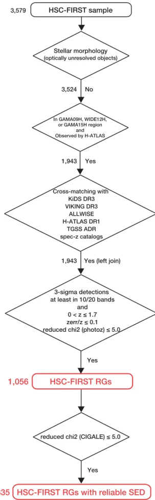
Figure1shows aflow chart of our sample selection process. The original sample was drawn from 3579 RGs and quasars in Yamashita et al. (2018), who used the HSC–SSP and FIRST
data. The HSC–SSP is an ongoing optical imaging survey with five broadband filters (g-, r-, i-, z-, and y-band) and four narrowbandfilters (see Aihara et al.2018a; Bosch et al.2018; Coupon et al.2018; Huang et al.2018). This survey consists of
three layers, Wide, Deep, and UltraDeep, and this work uses S16A Wide-layer data12 obtained from 2014 March to 2016 January, providing a forced photometry of g-, r-, i-, z-, and y-band with a 5σ limiting magnitude of 26.8, 26.4, 26.4, 25.5, and 24.7, respectively (Aihara et al. 2018b). The HSC–SSP
Wide-layer covers six fields (XMM-LSS, GAMA09H, WIDE12H, GAMA15H, HECTOMAP, and VVDS; see Table 1 in Yamashita et al. (2018) for detailed coordinates of each
field). The typical seeing is about 0 6 in the i-band, and the astrometric uncertainty is about 40 mas in root mean square (rms). Taking into account the photometric and astrometric flags, Yamashita et al. (2018) eventually extracted 23,795,523
HSC objects in the 154 deg2 for cross-matching with FIRST (see Section 2.1 in Yamashita et al.2018for more detail).
The FIRST project completed radio imaging survey at 1.4 GHz with a spatial resolution of 5 4(Becker et al. 1995; White et al.1997) covering 10,575 deg2, which is completely overlapping with the survey footprint of the HSC–SSP Wide-layer, and the final release catalog of FIRST (Helfand et al.
2015) is publicly available. Before cross-matching with the
HSC, Yamashita et al. (2018) made a flux-limited FIRST
sample with flux density at 1.4 GHz greater than 1.0 mJy. Taking into account a flag that tells a source is a spurious detection near a bright source, Yamashita et al. (2018)
eventually extracted 7072 FIRST objects in the 154 deg2for the cross-matching with the HSC(see Section 2.2 in Yamashita et al.2018for more detail). By cross-matching the HSC S16A Wide-layer catalog and FIRSTfinal data release catalog with a search radius of 1″, 3579 objects (including RGs and radio-loud quasars) were selected (see Section 3 in Yamashita et al.
2018for more detail).
12
The S16A data(Wide, Deep, and UltraDeep) is available in 2019 as a public data release 2(Aihara et al.2019). Although Yamashita et al. (2018) used UltraDeep data in addition to Wide data, this work focuses only on Wide data.
Before compiling multi-wavelength data, we made a parent RG sample. First, we removed 55 stellar objects (i.e., radio-loud quasars) based on optical morphological information (see Yamashita et al.2018). For 3579 − 55=3524 RGs, we then
narrowed down the sample to 2118 objects in threefields with a total area of ∼94.7 deg2 (GAMA09H, WIDE12H, and GAMA15H) where multi-wavelength data are available. We then removed 175 objects that are not covered by FIR observation (see Section 2.1.4), which yielded 1943 RGs.
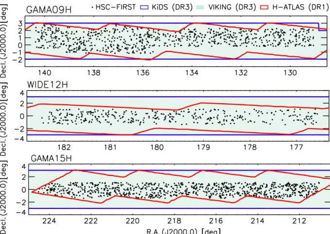
The sky distribution of those 1943 RGs is shown in Figure2. For those objects, we then complied the multi-wavelength data from u-band, near-IR(NIR), MIR, FIR, and radio data, as well as spectroscopic or photometric redshift. After removing 897 objects with photometric data less than 10, and unreliable photometric redshift and/or photometric redshift greater than 1.7(see Section2.1.6), we finally selected 1943 − 897=1056
objects(hereafter “HSC–FIRST RGs”) with multi-wavelength data and reliable redshift in this work.
2.1.1. u-band Data
The u-band data were taken from the Kilo-Degree Survey (KiDS; de Jong et al.2013),which is an ESO public survey carried
out with the VLT Survey Telescope (VST) and OmegaCAM camera (Kuijken 2011). We used the Data Release (DR) 3 (de
Jong et al.2017), which consists of 48,736,590 sources with a
limiting magnitude of 24.3 mag(5σ in a 2″ aperture) in u-band. The typical full width at half maximum(FWHM) of point-spread function (PSF) for u-band detected point sources is about 1″.13 Before the cross-matching, we extracted 42,252,797 sources with FLAG_U=0 to ensure clean photometry in u-band (see de Jong et al.2015,2017for more detail).
2.1.2. Near-IR Data
We compiled NIR data from the VISTA Kilo-degree Infrared Galaxy Survey (VIKING; Arnaboldi et al. 2007)
DR314 that includes 73,747,647 sources in ∼1000 deg2 with NIR taken by the VISTA InfraRed Camera(VIRCAM; Dalton et al.2006). We used J-, H-, and Ks-band with a median 10σ
(Vega)magnitude limit of 20.1, 19.0, and 18.6 mag, respec-tively. Objects with a PSF FWHM of<1 2 was observed in VIKING. Before the cross-matching, we selected 63,028,265 objects with primary_source=1 and (jpperrbits <256 or hpperrbits <256 or kspperrbits <256) to ensure clean photometry for uniquely detected objects(see also Toba et al.2015; Noboriguchi et al.2019).
2.1.3. Mid-IR Data
The MIR data were taken from Wide-field Infrared Survey Explorer (WISE; Wright et al. 2010). We utilized W1
(3.4 μm), W2 (4.6 μm), W3 (12 μm), and W4 (22 μm) data in ALLWISE(Cutri et al.2014) that consists of 747,634,026
sources. The 5σ detection limits15 in W1, W2, W3, and W4 band are approximately 0.054, 0.071, 0.73, and 5 mJy, respectively. The angular resolutions in W1, W2, W3, and W4 band are 6 1, 6 4, 6 5, and 12 0, respectively. We extracted
Figure 1.Flow chart of the sample selection process.
13http://kids.strw.leidenuniv.nl/DR3/catalog_table.php 14
http://eso.org/rm/api/v1/public/releaseDescriptions/107 15
741,753,366 sources with (w1sat=0 and w1cc_map=0) or (w2sat=0 and w2cc_map=0) or (w3sat=0 and w3cc_map=0), or (w4sat=0 and w4cc_map=0) in the ALLWISE catalog (Cutri et al. 2014), to have secure
photometry at either band(see the Explanatory Supplement to the ALLWISE Data Release Products16for more detail).
2.1.4. Far-IR Data
We also used FIR data that were provided by a project of the Herschel Space Observatory(Pilbratt et al.2010) Astrophysical
Terahertz Large Area Survey (H-ATLAS; Eales et al. 2010; Bourne et al.2016). The data were taken with the Photoconductor
Array Camera and Spectrometer(PACS; Poglitsch et al.2010) at
100 and 160μm and with the Spectral and Photometric Imaging REceiver instrument(SPIRE; Griffin et al.2010) at 250, 350, and
500μm. The typical PSF FWHMs of 100, 160, 250, 350, and 500μm are 11 4, 13 7, 17 8, 24 0, and 35 2, respectively. We used H-ATLAS DR1 (Valiante et al. 2016) containing 120,230
sources in the galaxy and mass assembly(GAMA) fields. The 1σ noise for source detection (that includes confusion and instru-mental noise) is 44, 49, 7.4, 9.4, and 10.2 mJy at 100, 160, 250, 350, and 500μm, respectively (Valiante et al.2016).
2.1.5. Ancillary Radio Data
The radio data were taken from observations with the Giant Metrewave Radio Telescope(GMRT; Swarup1991). We used
continuumflux density at 150 MHz (∼1.99 m) provided by the Tata Institute of Fundamental Research (TIFR) GMRT Sky Survey (TGSS) alternative data release (ADR; Intema et al.
2017), which includes 623,604 radio sources in 36,900 deg2. The median rms noise of sources is 3.5 mJy beam−1, with a spatial resolution of about 25″.
2.1.6. Cross-identification of Multi-band Catalogs
We then cross-identified those catalogs (KiDS, VIKING, ALLWISE, H-ATLAS, and TGSS) with HSC–FIRST RGs.17 By using a search radius of 1″ for KiDS and VIKING, 3″ for ALLWISE, 10″ for H-ATLAS, and 20″ for TGSS, 1051 (54.1%), 1564 (80.5%), 1482 (76.3%), 257 (13.2%), and 471 (24.2%) objects were cross-identified by KiDS, VIKING, ALLWISE, H-ATLAS, and TGSS, respectively. We note that 3/1051 (∼0.3%) and 2/471 (∼0.4%) objects have two candidates of counterpart for VIKING and TGSS sources, respectively, within the search radius. We choose the nearest object as a counterpart for such cases. For cross-matching with other catalogs(KiDS, ALLWISE, and H-ATLAS), one-to-one identification was realized. The matches by chance coincidence are estimated by generating mock catalogs with random positions, in the same manner as Yamashita et al.(2018). We
generated mock catalogs of KiDS, VIKING, ALLWISE, H-ATLAS, and TGSS data where source position in each catalog is shifted from the original one to±1° or ±2° along the
Figure 2.Spatial distribution(J2000.0) of 1943 HSC–FIRST radio galaxies (black points) in GAMA09H (top), WIDE12H (middle), and GAMA15H (bottom) field. Blue, green, and red squares represent survey footprint of KiDS, VIKING, and H-ATLAS, respectively. Those regions are completely covered by ALLWISE and TGSS. There are 754, 344, and 845 HSC–FIRST objects in the GAMA09H, WIDE12H, and GAMA15H, respectively.
16
http://wise2.ipac.caltech.edu/docs/release/allwise/expsup/index.html
17
We always use right assignation and decl. in the HSC catalog as coordinates of HSC–FIRST objects.
right assignation direction(see Yamashita et al.2018for more detail). We then cross-identified HSC–FIRST RGs with those mock catalogs with the exactly same search radii. We found that the chance coincidence of cross-matching with the KiDS, VIKING, ALLWISE, H-ATLAS, and TGSS catalogs is about 5.0%, 1.9%, 3.4%, 9.3%, and 0.6%, respectively.
We also compiled photometric and spectroscopic redshift. For spectroscopic redshift, we utilized the SDSS DR12(Alam et al.2015), the GAMA project DR2 (Driver et al.2011; Liske et al. 2015), and WiggleZ Dark Energy Survey project DR1
(Drinkwater et al. 2010). For photometric redshift, we
employed a custom-designed Bayesian photometric redshift code (MIZUKI; Tanaka 2015) to estimate the photometric
redshift (photo-z) of HSC–FIRST objects in the same manner as Yamashita et al. (2018), in which we used zbest as a
photometric redshift (see also Tanaka et al.2018). In order to
perform an accurate SED fitting, we preferentially used spectroscopic redshift. For objects without spectroscopic redshift, we used their zbestif they have a reliable photometric
redshift, i.e., 0<zbest1.7,18 szbest zbest0.1, and reduced
χ2
of zbest 5.0. These criteria are optimized based on the
comparison with spectroscopic redshift for the WERGS sample in Yamashita et al. (2018) (see also Tanaka et al. 2018).
However, the influence of the above criteria on physical quantities derived from the SEDfitting is still unclear, which will be discussed in Section 4.2.1. In addition to the above redshift(quality) cut, we extracted objects with >3σ detection in at least 10 photometric bands among 20 photometric data (u, g, r, i, z, y, J, H, Ks-band; 3.4, 4.6, 12, 22, 100, 160, 250,
350; 500μm; and 150 and 1400 MHz) to avoid an overfitting for our SED fitting method (see Section 2.2). Consequently,
1056 HSC–FIRST RGs with multi-band photometry and reliable redshift were left(see Figure1). Among 1056 objects,
the redshifts of 224, 44, and 3 objects were taken from the SDSS DR12, GAMA DR2, and WiggleZ DR1, respectively, while the redshifts of the remaining 785 objects were taken from MIZUKI. The HSC–FIRST RG catalog, which includes basic information such as redshift and multi-band photometry, is accessible through an online service. Format and column descriptions of the catalog are summarized in Table3.
2.2. SED Modeling withCIGALE
We here employed CIGALE19(Code Investigating GALaxy Emission; Burgarella et al. 2005; Noll et al. 2009; Boquien et al.2019) in order to perform a detailed SED modeling in a
self-consistent framework with considering the energy balance between the UV/optical and IR. In this code, we are able to handle many parameters, such as star formation history(SFH), single stellar population(SSP), attenuation law, AGN emission, dust emission, and radio synchrotron emission.
We assumed an SFH of two exponential decreasing SFR with different e-folding times (Ciesla et al.2015, 2016). We
adopted the stellar templates provided from Bruzual & Charlot (2003) assuming the initial mass function (IMF) in Chabrier
(2003), and the standard default nebular emission model
included in CIGALE (see Inoue 2011). Dust attenuation is
modeled by using the Calzetti et al. (2000) law with color
excess(E(B−V )*). We note that even if we employ the dust attenuation law of the Small Magellanic Cloud that would be applicable to dusty starburst galaxies, resultant physical properties are consistent with what we present in this work within error. The reprocessed IR emission of dust absorbed from UV/optical stellar emission is modeled assuming dust templates of Dale et al. (2014). For AGN emission, we also
utilized models provided in Fritz et al.(2006), where we fixed
some parameters that determine the density distribution of the dust within the torus to avoid a degeneracy of AGN templates in the same manner as Ciesla et al.(2015). We parameterized
theψ parameter (an angle between the AGN axis and the line of sight) that corresponds to a viewing angle of the tours. We also parameterize AGN fraction ( fAGN), which is the
contrib-ution of IR luminosity from AGN to the total IR luminosity (Ciesla et al.2015). For radio synchrotron emission from either
SFG or AGN, we parameterized a correlation coefficient between FIR and radio luminosity(qIR) and the slope of
power-law synchrotron emission (αradio) (but see Sections3.5.6 and
3.5.7). We define αradiofrom the measured radioflux density at
observed-frame frequencies at 150 MHz and 1.4 GHz, assum-ing a power-law radio spectrum of fn µn-aradio;
a n n = log F F log . 1 radio 150 MHz 1.4 GHz 1.4 GHz 150 MHz ( ) ( ) ( )
This synchrotron emission is cut off at 100μm; that is, a default value adopted in CIGALE that would be optimized for normal star-forming galaxies. However, the synchrotron emission may contribute to fluxes/luminosities even at <100 μm, especially for radio-loud AGNs(e.g., Mason et al.2012; Privon et al.2012; Falkendal et al. 2019; Rakshit et al. 2019). In this work, we
choose 30μm as a cutoff wavelength of the synchrotron emission with a single power law, in the same manner as Lyu & Rieke(2018) (see also Pe’er2014). We have confirmed that
the choice of cutoff wavelength does not significantly affect the following results. Table 1 lists the detailed parameter ranges adopted in the SEDfitting (see also Matsuoka et al.2018; Chen et al.2019; Toba et al.2019). In addition to the energy balance
between UV/optical and IR part, CIGALE takes into account the balance between IR and radio luminosity that is parameterized by qIR, which are eventually an essential framework in CIGALE.
Tofind a best-fit SED and calculate physical properties and their uncertainties, CIGALE employed an analysis module so-called pdf_analysis. This module computes the likelihood (that corresponds to χ2) for all the possible combinations of
parameters and generates the probability distribution function (PDF) for each parameter and each object. But before computing the likelihood, the module scaled the models by a factor (α) to obtain physically meaningful values (so-called extensive physical properties) such as stellar masses and IR luminosities, whereα can be derived as follows:
å
å
å
å
a = s + s s s , 2 i f m i m j f m j m i i i i i j j j j j 2 2 2 2 2 2 ( )where fiand miare the observed and modelflux densities, fjand
mjare the observed and model extensive physical properties,
andσ is the corresponding uncertainties (see Equation (13) in Boquien et al.2019). Finally, pdf_analysis computes the
18
Yamashita et al. (2018) reported that the HSC–SSP photo-z derived by MIZUKIcould be secure at z1.7 based on comparison with spectroscopic redshift in COSMOSfield (see Section 5.1.2 in Yamashita et al.2018for more detail).
19
probability-weighted mean and standard deviation that corre-spond to resultant value and its uncertainty for each parameter, in whichα is considered as a free parameter. This approach is fully valid as far as one compares models built from the same set of parameters(see Section 4.3 in Boquien et al.2019for full explanation of this module) (see also, Salim et al.2007).
Under the parameter setting described in Table 1, we fit the stellar, AGN, SF, and radio components to at most 20 photometric points(u, g, r, i, z, y, J, H, Ks-band, and 3.4, 4.6, 12, 22, 100, 160,
250, 350, and 500μm, and 150 and 1400 MHz) of 1056 HSC– FIRST RGs observed with KiDS, HSC, VIKING, ALLWISE, H-ATLAS, FIRST, and TGSS. For optical data, we used MAG_AUTO_U as a u-band photometry that is a default magnitude20 while g/r/i/z/ycModel_Mag were used for g-, r-, i-, z-, and y-band photometry(Bosch et al.2018; Huang et al.2018). For NIR data, we used Petrosian (1976) magnitude
(see the release note of the VIKING DR3). Each magnitude was corrected for Galactic foreground extinction following Schlegel et al.(1998). The VIKING catalog contains the Vega
magnitude of each source, and we converted these to AB magnitude, using offset values Δm (mAB=mVega+Δm) for
J, H, and Ks-band of 0.916, 1.366, and 1.827, respectively.21
For MIR and FIR data, w1-4mpro were utilized to estimate MIRflux densities (Wright et al.2010; Toba et al.2014) while
F100/160/250/350/500BEST were used for FIR flux densities(see Valiante et al.2016). ALLWISE catalog contains
the Vega magnitude of each source, and we converted these to AB magnitude, usingΔm for 3.4, 4.6, 12, and 22 μm of 2.699, 3.339, 5.174, and 6.620, respectively.22 It is known thatflux densities at 250, 350, and 500μm could be boosted especially for faint sources(so-called flux boosting or flux bias) that are caused by a confusion noise and instrument noise. Hence we corrected this effect by using the correction term provided in Table 6 of Valiante et al. (2016). For radio data, FINT and
STOTALwere used forflux densities at 1.4 GHz and 150 MHz, respectively (see Helfand et al. 2015; Intema et al. 2017 for more detail). We used flux density at a wavelength when signal-to-noise ratio(S/N) is greater than 3 at that wavelength. If an object was undetected, we put 3σ upper limits at those wavelengths.23 Although the photometry employed in each catalog is different, theirflux densities are expected to trace the total flux densities. Therefore, the influence of different photometry is likely to be small. Nevertheless, it is worth investigating whether or not physical properties can actually be estimated in a reliable way given an uncertainty of each photometry, which will be discussed in Section4.2.4.
3. Results
3.1. Histogram of i-band Magnitude and Redshift Figure3 shows a histogram of i-band magnitude for 1056 HSC–FIRST RGs. Here, we define the “SDSS-level objects” and “HSC-level objects” based on the Galactic foreground extinction-corrected i-band magnitude in the same manner as Yamashita et al.(2018). We call objects with <i 21.3 mag the SDSS-level objects as a reference of optically bright RGs, while we call objects with i 21.3 mag the HSC-level objects as a reference of optically faint RGs. We found that 577 and 479 objects are classified as the SDSS-level and HSC-level objects, respectively, meaning that we have a statistically
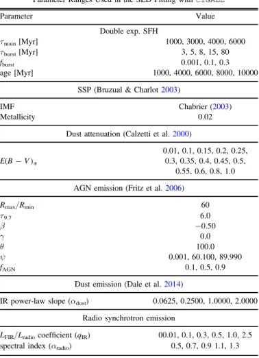
Table 1
Parameter Ranges Used in the SED Fitting with CIGALE
Parameter Value Double exp. SFH τmain[Myr] 1000, 3000, 4000, 6000 τburst[Myr] 3, 5, 8, 15, 80 fburst 0.001, 0.1, 0.3 age[Myr] 1000, 4000, 6000, 8000, 10000
SSP(Bruzual & Charlot2003)
IMF Chabrier(2003)
Metallicity 0.02
Dust attenuation(Calzetti et al.2000)
0.01, 0.1, 0.15, 0.2, 0.25,
E(B−V )* 0.3, 0.35, 0.4, 0.45, 0.5,
0.55, 0.6, 0.8, 1.0 AGN emission(Fritz et al.2006)
Rmax/Rmin 60 τ9.7 6.0 β −0.50 γ 0.0 θ 100.0 ψ 0.001, 60.100, 89.990 fAGN 0.1, 0.5, 0.9
Dust emission(Dale et al.2014)
IR power-law slope(αdust) 0.0625, 0.2500, 1.0000, 2.0000
Radio synchrotron emission
LFIR/Lradiocoefficient (qIR) 00.01, 0.1, 0.3, 0.5, 1.0, 2.5
spectral index(αradio) 0.5, 0.7, 0.9 1.1, 1.3
Figure 3.Histogram of i-band magnitude of HSC–FIRST RGs (black line) and those with reducedχ2of the SEDfitting smaller than 5.0 (gray region), where i-band magnitude is corrected for the Galactic foreground extinction (see Section2.2). The vertical dashed line is the threshold (i=21.3 mag) between SDSS-level and HSC-level RGs.
20http://www.eso.org/rm/api/v1/public/releaseDescriptions/82 21 http://casu.ast.cam.ac.uk/surveys-projects/vista/technical/filter-set 22 http://wise2.ipac.caltech.edu/docs/release/allsky/expsup/sec4_4h.html# conv2ab 23
CIGALEcan handle SEDfitting of photometric data with upper limit when one employs the method presented by Sawicki(2012). This method computes χ2by introducing the error function(see Equations (15) and (16) in Boquien
robust sample of optically faint RGs that are newly discovered by the WERGS project(Yamashita et al.2018).
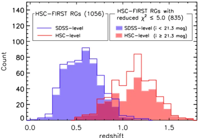
Figure4shows a histogram of redshift for 1056 HSC–FIRST RGs. The mean values of redshift for the SDSS- and HSC-level objects are 0.57 and 1.10, respectively, meaning that HSC-level objects have larger redshift than SDSS-level objects, which is consistent with what Yamashita et al. (2018) reported.
3.2. Result of SED Fitting
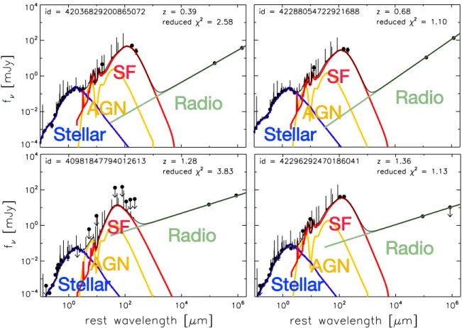
Figure5shows examples of the SEDfitting with CIGALE.24 We confirmed that 568/1056 (∼54%) objects have reduced χ23.0, while 835/1056 (∼79%) objects have reduced
χ25.0, which means that the data are moderately well fitted
with the combination of the stellar, AGN, SF, and radio components by CIGALE.
We note that each quantity derived by the SEDfitting would not be uniquely determined for some objects even if their reduced χ2 is good enough, because there is a possibility of degeneracy among input parameters. We checked the PDF of each quantity for randomly selected objects. We confirmed that there is basically no prominent secondary peak of their PDFs, suggesting that the derived physical quantities are reliably determined. The physical quantities such as stellar mass and SFR for 1056 HSC–FIRST RGs are also accessible through the online service(see Table3for the catalog description).
3.3. Radio and Optical Luminosity as a Function of Redshift Figure 6(a) shows the rest-frame 1.4 GHz radio luminosity
(L1.4 GHz) of 835 HSC–FIRST RGs as a function of redshift. To
make sure of the parameter space of our RGs with respect to previously discovered RGs, RGs selected with the SDSS(Best & Heckman 2012) and RGs found by VLA-COSMOS 3 GHz
large project (Smolčić et al. 2017a, 2017b) are also plotted.
L1.4 GHz in unit of W Hz−1 is k-corrected luminosity at
rest-frame 1.4 GHz, which is derived by using the following
formula: p = + -a L d F z 4 1 , 3 L 1.4 GHz 2 1.4 GHz 1 radio ( ) ( )
where dLis luminosity distance, F1.4 GHzis observed-frameflux
density at 1.4 GHz, and αradio is the radio spectral index we
estimated in Equation(1). We note that 190/835 objects have
TGSS (150 MHz) data and thus their αradio are securely
estimated. If an object did not have αradio due to the
non-detection of TGSS, we adopted a typical spectral index of RGs, αradio=0.7 (e.g., Condon1992) to estimate L1.4 GHz. For radio
sources selected with either the SDSS or VLA-COSMOS, we also used 0.7 as the spectral index to calculate L1.4 GHz if the
object did not have radio spectral index(see e.g., Smolčić et al.
2017a). We confirmed that our RG sample distributes much
higher redshift(z>0.5) than SDSS-selected RGs, while radio luminosity of our RGs sample is larger than that of VLA-COSMOS radio sources, with a median rms of 2.3μJy beam−1. Figure6(b) shows the rest-frame i-band absolute magnitude
(Mi) as a function of redshift. Mi of our RG sample was
estimated based on the best-fit SED output by CIGALE. Since the VLA-COSMOS catalog (Smolčić et al. 2017a) does not
contain Mi, we used the COSMOS2015 catalog (Laigle et al.
2016), in which absolute magnitudes in optical and NIR bands
were estimated based on the SEDfitting. For SDSS-selected RGs in Best & Heckman(2012), we did not apply for k-correction. But
their Mican be approximately used for absolute magnitude at the
rest frame because they are low-z objects. We confirmed that our RG sample has intermediate value of Mibetween SDSS-selected
and VLA-COSMOS radio sources.
The discrepancy between our RG sample and VLA-COSMOS RG sample in Mi (Figure 6(b)) is much smaller
than that in L1.4 GHz(Figure6(a)), suggesting that our RGs tend
to trace higher radio-loudness sources, which is one of the advantages of the WERGS project, where even VLA-COSMOS might not be able to trace. In summary, Figure 6
reminds us that our RG survey with HSC and FIRST explores a new parameter space: relatively high-z luminous RGs. We should keep in mind the above parameter space in the following discussions.
3.4. WISE Color–Color Diagram
Figure7 shows the WISE color–color diagram ([3.4]–[4.6] versus[4.6]–[12]) for 148 HSC–FIRST RGs with S/N>3 in 3.4, 4.6, and 12μm that were drawn from 1056 RG sample. The anticipated MIR colors for various populations of objects are shown with different colors (Wright et al. 2010), which
provides us a qualitative view of galaxies. We found that the HSC-level objects tend to be redder than the SDSS-level objects in both colors of [3.4]–[4.6] and [4.6]–[12]. The majority of the SDSS-level objects is located at regions of spirals and LIRGs, while the HSC-level objects are located at regions of Seyferts, starburst galaxies, and ULIRGs.
About 49% of HSC–FIRST RGs with S/N>3 in 3.4, 4.6, and 12μm are located within the AGN wedge defined by Mateos et al.(2012,2013), who suggested reliable MIR color
selection criteria for AGN candidates based on the WISE and wide-angle Bright Ultrahard XMM-Newton survey (BUXS: Mateos et al. 2012). This means that roughly half of the RG
sample is outside of the wedge, which is in good agreement
Figure 4.Histogram of redshift of HSC–FIRST RGs (solid line) and those with reducedχ2of the SEDfitting smaller than 5.0 (shaded region). Red and blue line are the SDSS- and HSC-level objects in 1056 HSC–FIRST RGs. Red and blue regions are those in the 835 subsample(see Section3.5).
24
Since CIGALE assumed that the maximum wavelength for radio data was rest frame 1 m, CIGALE did not work for our data set, including TGSS(2 m) data for low-z objects. We modified CIGALE code (radio.py) to solve this issue as suggested by Prof. Denis Burgarella through a private communication.
with previous works on radio-loud galaxies (Gürkan et al.
2014; Banfield et al.2015), suggesting that the AGN selection
based on the AGN wedge seems to be biased toward a subsample among the entire AGN population (see also Toba et al.2014,2015; Ichikawa et al.2017).
What makes the difference between objects inside and outside of the AGN wedge? One possibility is a difference of radio luminosity between them, since radio luminosity is a good tracer of AGN power, as suggested by previous works (e.g., Banfield et al. 2015; Singh et al. 2015; Singh & Chand 2018). We checked this possibility for our sample,
where we used the rest-frame radio luminosity at 1.4 GHz that is drawn from Yamashita et al.(2018) assuming a power-law
radio spectrum of fν∝ν−0.7.
Figure 7 shows the histogram of rest-frame 1.4 GHz luminosity, indicating a systematic difference in radio lumin-osity for objects inside and outside of the AGN wedge. The mean values of rest-frame 1.4 GHz luminosity for objects inside and outside of the AGN wedge are logL1.4 GHz~24.8 and ∼24.4 W Hz−1, respectively, supporting the previous works. An alternative indicator of AGN power is a radio-loudness that is defined as flux ratio of rest-frame radio and optical band. We used the radio-loudness at rest frame(Rrest), a
ratio of the rest-frame 1.4 GHz flux to the rest-frame g-band flux as used in Yamashita et al. (2018). Figure7also shows the histogram of Rrest, indicating a systematic difference in Rrestfor
objects inside and outside of the AGN wedge. The mean values of Rrestfor objects inside and outside of the AGN wedge are
~
R
log rest 2.4 and ∼1.9, respectively, indicating that objects
Figure 5.Examples of the SED(flux density as a function of wavelength in rest frame) and result of the SED fitting for our sample. The black points are photometric data where the down arrows mean 3σ upper limit. The blue, yellow, red, and green lines show stellar, AGN, SF, and radio component, respectively. The black solid lines represent the resultant SEDs. We provide best-fit SEDs for all 1056 HSC–FIRST RGs with derived physical properties (see Tables3and4).
Figure 6.(a) Rest-frame 1.4 GHz radio luminosity and (b) the absolute i-band magnitude at the rest frame as a function of redshift. Yellow and blue circles represent SDSS-detected RGs(Best & Heckman2012) and RGs discovered by the VLA-COSMOS project(Smolčić et al. 2017a), respectively. Red circles represent HSC–FIRST RGs with reduced χ2 5.0.
with larger radio-loudness tend to be located in the AGN wedge, as we expected.
We note that there are almost no objects at elliptical galaxies in the WISE color–color diagram (Figure 7), which is mainly
interpreted as a selection bias of our HSC–FIRST RGs. Since the saturation limit of the HSC for point sources at r-band and i-band are 17.8 and 18.4 mag, respectively (Aihara et al. 2018b), the
HSC–FIRST RG sample does not contain those optically bright objects. In Figure 7, we also plot RGs with r-band magnitude smaller than 17.8 mag provided by Capetti et al.(2017a,2017b),
who released Fanaroff & Riley(1974) (FR) I and II RG catalogs25
selected with the SDSS and FIRST. The redshift, optical
absolute magnitude, and radio luminosity range of those RGs are 0.02<z<0.15, −23.7<MR<−20.3, and23.3<
<
-L
log 1.4 GHz[W Hz 1] 25.8, respectively. They show ellip-tical-like MIR colors, which means that optically too bright objects are located at the region of elliptical galaxies. In addition to the selection bias, there is a possibility that MIR colors of RGs would be different from normal elliptical galaxies. Banfield et al. (2015) reported that [4.6]–[12] color of RGs selected from the
Radio Galaxy Zoo26sample shows significantly redder than that of typical elliptical galaxies. This indicates that the dust emission of RGs may be enhanced compared with normal quiescent elliptical galaxies(see also Goulding et al.2014; Gürkan et al.
2014). Indeed, Martini et al. (2013) reported that active elliptical
Figure 7.(Top) WISE color–color diagram of 148 HSC–FIRST RGs with S/N>3 in 3.4, 4.6, and 12 μm. Blue and red circles are SDSS- and HSC-level RGs, respectively. Yellow and green circles are SDSS-detected FIRST FRI and FRII RGs with r<17.8 mag, respectively, that are obtained from Capetti et al. (2017a,2017b). Regions with different color shading show typical MIR colors of different populations of objects (Wright et al.2010). The solid lines illustrate the AGN selection wedge defined from Mateos et al. (2012,2013). (Bottom) Histogram of rest-frame 1.4 GHz luminosity (L1.4 GHz) and rest-frame radio-loudness (Rrest)
for objects inside(magenta) and outside (black) of the AGN wedge. The mean values are shown in dashed lines.
25
Since the catalogs do not contain WISE magnitudes, we cross-identified
galaxies tend to have a large dust mass compared with inactive elliptical galaxies, which supports the above hypotheses.
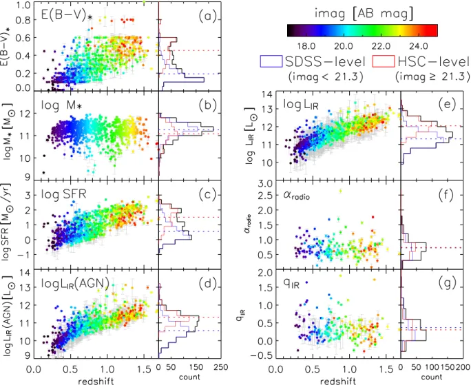
3.5. Physical Properties of HSC–FIRST Radio Galaxies We present the physical properties of HSC–FIRST RGs with being conducted a reliable SEDfitting. Hereafter, we will focus on a subsample of 835 HSC–FIRST RGs with reduced χ2of the SEDfitting smaller than 5.0. In this work, we investigate the following quantities output directly from CIGALE;(i) dust extinction,(ii) stellar mass, (iii) SFR, (iv) AGN luminosity, (v) IR luminosity, and those calculated by ourselves; (vi) radio spectral index, and (vii) LIR/Lradio coefficient (qIR) as a
function of redshift, which are summarized in Figure 8. Among subsample, 501 and 334 objects are classified as the SDSS- and HSC-level objects with a mean redshift of 0.56 and 1.11, respectively (see Figures3and4).
3.5.1. Dust Extinction
Figure8(a) shows color excess, E(B−V )*as a function of redshift, where E(B−V )*is an indicator of dust extinction of host galaxy. We found that there is a clear correlation between redshift and E(B−V )*; optically fainter RGs at high redshift
are affected by larger dust extinction. The mean values of E(B−V )*of the SDSS- and HSC-level objects are∼0.19 and ∼0.45, respectively. Indeed, 5 HSC-level objects with mean E(B−V )*of 0.45 satisfy a criterion of IR-bright dust-obscured galaxies with S/N>3 at 22 μm (see e.g., Toba et al. 2015; Toba & Nagao2016; Toba et al.2017b,2018; Noboriguchi et al.
2019).
3.5.2. Stellar Mass
Figure8(b) shows stellar mass as a function of redshift. The
stellar mass of our RG sample does not significantly depend on redshift, and thus the distributions of stellar masses for the SDSS- and HSC-level objects are similar. However, the mean values of stellar mass of the SDSS- and HSC-level objects are
~
M M
log( * ☉) 11.26and∼11.08, respectively, indicating that the HSC-level RGs could tend to have less massive stellar mass compared with the SDSS-level ones.
3.5.3. Star Formation Rate(SFR)
Figure8(c) shows SFR as a function of redshift. We found
that the SFR increases with increasing redshift, and thus the HSC-level objects are systematically larger than those of the
Figure 8.(a) The color excess (E(B−V )*), (b) stellar mass, (c) SFR, (d) IR luminosity contributed from AGNs, (e) total IR luminosity, (f) radio spectral index (αradio), and (g) qIRof HSC–FIRST RGs as a function of redshift. The color code is i-band magnitude. The histograms show the SDSS-level (blue), HSC-level (red),
and total(black) objects. The dashed lines are mean values of each quantity for SDSS-level (blue) and HSC-level (red) objects. 835 RGs are plotted in panels (a) to (e) while 190 RGs with FIRST and TGSS data are plotted in panels (f) and (g).
SDSS-level objects. The mean values of SFR of the SDSS- and HSC-level objects are log SFR ∼0.55 and ∼1.51 M☉ yr−1, respectively. About one-quarter of the HSC-level objects have SFR >100 M☉ yr−1, which is consistent with what was reported in the WISE color–color diagram (Figure7).
3.5.4. AGN Luminosity
Figure8(d) shows IR luminosity contributed from AGN that
is defined as LIR(AGN)=fAGN×LIR (Ciesla et al. 2015),
where LIRis total IR luminosity(see Section3.5.5). We found
that the LIR(AGN) increases with increasing redshift, and thus
the HSC-level objects seem to have systematically larger AGN luminosity than the SDSS-level objects. The mean values of
L
log[ IR (AGN)/L ]☉ of the SDSS- and HSC-level objects are
∼10.56 and ∼11.32, respectively. 3.5.5. IR Luminosity
Figure 8(e) shows IR luminosity as a function of redshift.
We can see a similar trend to AGN luminosity; IR luminosity increases with increasing redshift, and thus IR luminosities of the HSC-level objects are larger than those of the SDSS-level objects. The mean values of log(LIR L☉) of the SDSS- and
HSC-level objects are ∼11.31 and ∼12.04, respectively. This is basically consistent with the fact that the majority of the SDSS and HSC objects are LIRGs and ULIRGs, respectively, reported in Section3.4.
We note that because our RG sample may be affected by Malmquist bias as shown in Figure 6, the difference particularly in SFR, LIR (AGN), and LIR between SDSS- and
HSC-level objects is basically due to the difference of their redshift distributions. In other words, redshift dependence of LIR, LIR(AGN), and SFR may be caused by the sensitivity limit
of IR bands. On the other hand, it is natural that M*does not show a redshift dependence, because the sensitivity of optical bands with HSC is much deeper than that of the IR bands. If we compare SFR, LIR (AGN), and LIR of SDSS- and HSC-level
objects at an overlapped redshift range (0.5<z< 1.0) (see Figure4), the differences of mean values of SFR, LIR(AGN),
and LIRare 0.31, 0.30, and 0.25 dex, respectively. We also note
that particularly SFR and AGN luminosity would also have an additional uncertainty probably due to a poor constraint of SED given a limited number of data points in MIR and FIR (see Section 4.2.4).
3.5.6. Radio Spectral Index
We present radio spectral index (αradio) and luminosity
ratio of IR and radio wavelength (qIR) in the following
subsections. Although our sample always has 1.4 GHz data, only one-quarter of objects have 150 MHz data as reported in Section2.1.6. This means that it is quite hard to determine the radio properties with CIGALE for objects without counter-parts of TGSS given a limited number of data points and input parameters. Indeed, the radio spectral index and qIR can
be analytically derived by assuming a radio spectrum. So, we focus on 190 HSC–FIRST RGs with both 1.4 GHz and 150 MHzflux densities in Sections3.5.6 and3.5.7.
We derive the radio spectral index (αradio) based on
Equation (1). Figure 8(f) shows radio spectral index as a
function of redshift. There is no clear correlation between αradio and redshift, which is consistent with previous works
(Blundell et al.1999; Bornancini et al.2010; Calistro Rivera et al. 2017). The mean value of αradio of 190 HSC–FIRST
RGs is∼0.73, which is consistent with what was reported in de Gasperin et al. (2018), who investigated radio spectral
index over 80% of the sky based on the NVSS and TGSS. The mean values ofαradioof the SDSS- and HSC-level objects are
∼0.72 and ∼0.74, respectively. De Gasperin et al. (2018)
reported that the absolute value of radio spectral index increases with radio flux densities. Because radio flux densities at 150 MHz and 1.4 GHz of the HSC-level objects are slightly larger than those of SDSS-level objects, the tiny difference of αradio between SDSS- and HSC-level objects
could be explained as a difference of their radioflux densities. 3.5.7. qIR
The ratio of IR and radio luminosity (qIR) is defined as
follows(see also Helou et al.1985; Ivison et al.2010):
= ´ q L L log 3.75 10 , 4 IR IR 12 1.4 GHz ( ) ⎛ ⎝ ⎜ ⎞⎠⎟
where LIRis the total IR luminosity in unit of W derived from
CIGALE. 3.75×10¹¹ is the frequency(Hz) corresponding to 80μm, which is used for making qIRa dimensionless quantity.
L1.4 GHz in unit of W Hz−1 is k-corrected luminosity at
rest-frame 1.4 GHz, which is derived by Equation(3).
Figure8(g) shows qIRas a function of redshift. Although there
is no clear dependence of qIRon redshift, the mean value of 190
HSC–FIRST RGs is 0.34, which is significantly lower than that of pure SF galaxies whose qIRis∼2–3 (Yun et al.2001; Bell2003;
Ivison et al.2010). This is reasonable because it is known that
radio-loud galaxies/AGNs withlogLradio>24W Hz−1tend to have significantly small qIR with wide dispersion (Sajina et al.
2008; Calistro Rivera et al.2017; Williams et al.2018). We will
discuss this point later by using “radio-excess parameter” in Section4.5.
The mean values of qIRof SDSS- and HSC-level objects are
∼0.37 and ∼0.31, respectively. Calistro Rivera et al. (2017)
reported that qIR could be decreased with increasing redshift,
while Read et al. (2018) reported that qIR could also be
decreased with increasing specific SFR (sSFR ≡ SFR/M*). Because HSC-level objects are located at higher redshift and they have smaller stellar mass and higher SFR (i.e., higher sSFR), as mentioned in Sections3.5.2and3.5.3, the difference in qIRbetween SDSS- and HSC-level objects may be explained
by the difference of their redshift and sSFR. 3.6. Composite Spectrum
Finally, we show a composite spectrum of the SDSS- and HSC-level objects in Figure9. Here we performed the median stacking only for 190 HSC–FIRST RGs with reliable radio spectral index. In optical to NIR regime, HSC-level objects are typically less luminous compared with SDSS-level objects, suggesting that HSC-level objects are more affected by dust extinction and their stellar masses are smaller than those of the SDSS-level objects, as reported in Sections 3.5.1 and 3.5.2. Once wavelength is beyond 1μm, hot dust emission heated by AGNs and cold dust emission heated by SF will be dominant for HSC-level objects, indicating that HSC-level objects have a large AGN and SF luminosity(i.e., large IR luminosity and SFR)
compared with SDSS-level objects, as reported in Sections
3.5.3–3.5.5. The best-fit SED template of each HSC–FIRST RG is available in Table4.
4. Discussion 4.1. Selection Bias
As described in Sections2 and3, we selected 1056 objects with reliable redshift and reasonable redshift cut among 1943 RGs and eventually investigated physical properties for 835 RGs with SED fitting. This means that 1943 − 835=1108 (∼57%) objects were excluded in this work, which would affect the results we presented above.
To check whether or not we would select a specific population among the entire HSC–FIRST RG sample, we investigated their optical colors. Figure10shows a color–color diagram of r−i versus i−z for the entire sample of 1943 objects and subsample of 835 objects. Because the HSC– FIRST RG sample requires all the detections of r, i, and z-band with S/N>5 (see Yamashita et al. 2018), all objects in the
entire sample and subsample are plotted in thisfigure. A two-sided K-S test does not rule out a hypothesis that the distribution of i−z for the subsample of 835 RGs is the same as that for the entire sample of 1943 RGs at >99.9% significance, which is also supported by a Wilcoxon rank-sum test. On the other hand, those two tests find that two distributions of r−i are statistically different. This could suggest that physical quantities of the subsample of 835 RGs may be (more or less) affected by selection bias, which we should keep in mind in the following discussions.
4.2. Possible Uncertainties
We discuss the possible uncertainties of physical properties derived by CIGALE. We consider the following four things: how (i) the uncertainty of photometric redshift and (ii) the difference in spatial resolution of each catalog affect the derived physical quantities, and comparison of resultant physical quantities with (iii) spectroscopically derived ones and(iv) those derived from the mock catalog. We find that our RG sample is likely to have additional uncertainties, especially for SFR and AGN luminosity. However, it is hard to estimate the exact uncertainty for an individual object because we infer
the additional uncertainty based on a sort of Monte Carlo simulation. Therefore, we do not include/propagate those possible uncertainties to the original ones output by CIGALE, and focus on a statistical view of possible uncertainties.
4.2.1. Uncertainty of Photometric Redshift
We selected 1056 HSC–FIRST RGs with reliable redshifts as described in Section 2. In particular, we allowed relative errors of photo-z to be at most 10%. Here we discuss how the uncertainty of photo-z affects the derived physical quantities with SED fitting, by performing the following test. First, we assumed a Gaussian distribution with a mean(a photo-z of an object) and sigma (its photo-z error) for each object, and randomly chose one value among the distribution as an adopted redshift. We then conducted the SED fitting with CIGALE under the exact same parameter as what we used in this work for 785 objects whose redshifts came from photo-z with MIZUKI(see Section2.1.6).
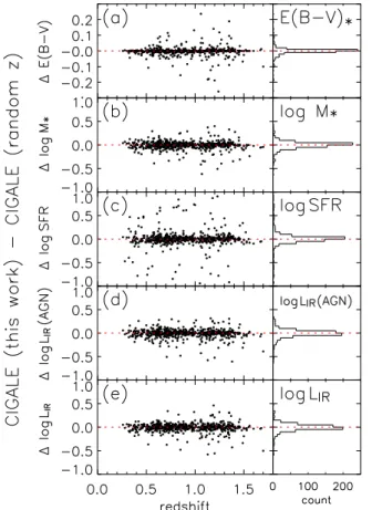
Figure11shows the differences in E(B−V )*,logM*, log
SFR,logLIR(AGN), andlogLIR derived from CIGALE in this
work and those derived from CIGALE with random redshift assuming a Gaussian for each object as a function of redshift. The mean values of each quantity are almost zero, while the standard deviations of DE B( -V *) , DlogM*, Δlog SFR,
Δlog LIR (AGN), and DlogLIRare 0.03, 0.09, 0.25, 0.10, and
0.10, respectively. We found thatΔlog SFR is slightly larger than others due to a relatively large fraction of outliers, suggesting that SFR is most sensitive to uncertainty of photometric redshift. We should keep in mind these possible uncertainties caused by photo-z error.
4.2.2. Influence of Difference in Spatial Resolution of Each Catalog on Physical Quantities
As described in Section2, we combined multi-wavelength catalogs with different spatial resolutions. In particular, because the angular resolutions of Herschel and GMRT are relatively poor, we adopted 10″ and 20″ as a search radius to cross-identify with H-ATLAS and TGSS, respectively. If there are multiple IR/radio sources within the search radii but H-ATLAS/TGSS could not resolve them, their FIR and radio (150 MHz) flux densities could be overestimated, which
Figure 9. Composite SEDs of SDSS-(blue) and HSC-level (red) RGs with reliable αradio. Shared regions represent standard deviation of the median
stacking SEDs. These SED templates are available in Table4.
Figure 10.Color–color diagram of r−i and i−z. The 1943 HSC–FIRST RG sample, and 835 RGs whose physical properties are studied in this work, are shown in black and magenta circles, respectively. Histogram of each color is also shown with solid lines(an entire sample of 1943 objects) and magenta-shaded regions(a subsample of 835 objects).
induces a systematic offset for physical quantities, such as IR luminosity and radio spectral index, that are derived by SED fitting (see e.g., Pearson et al. 2018). This effect would be
severe for fainter objects at high-z universe (i.e., HSC-level RGs). If we could deblend those sources and re-measure FIR and radio flux densities for an individual object, it would provide us (more or less) an accurate measurement of flux density, although the deblending process may also have an uncertainty, which is beyond the scope of this paper. Therefore, we briefly discuss a possible influence of relatively large beam sizes of H-ATLAS and TGSS on derived physical quantities.
First, we check a possibility of overestimate of FIR flux densities in H-ATLAS by using the ALLWISE catalog, whose sensitivity and angular resolution are better than those of Herschel (see Section 2.1.3). We count all nearby WISE
sources around an object with a search radius of 10″. If more than one WISE source is found around that object, those IR sources would contribute to FIR flux densities that are unresolved by Herschel, and their FIR flux densities would be overestimated. We confirm that 89/835 (∼11%) objects have multiple WISE counterparts within 10″. Here we test whether or not their IR luminosity has a systematically large value due to boost of their FIR flux densities.
Figure12shows the histogram of IR luminosity for 835 HSC– FIRST RGs and 89 objects with multiple WISE counterparts. We find that there is no systematic difference between them. The mean IR luminosity of 89 objects is log(LIR L☉)~11.48,
which is in good agreement with that of all HSC–FIRST RGs, suggesting that poor angular resolution of H-ATLAS does not significantly affect the measurement of FIR flux densities.
Next, we check a possibility of overestimate of radio flux density at 150 MHz in TGSS by using the FIRST catalog, whose sensitivity and angular resolution (6″) are better than those of GMRT. We count all nearby FIRST sources around an object with a search radius of 20″, and confirm that 27/190 (∼14%) objects have multiple FIRST counterparts within 20″. Here we test whether or not their radio spectral index (αradio) have
systematically large value due to a boost of their 150 MHzflux densities. Figure13shows the histogram of radio spectral index for 190 HSC–FIRST RGs, and 27 objects with multiple FIRST counterparts. Wefind that 27 objects systematically have large αradio. Their mean αradio is 1.19, which is significantly larger
than that of all HSC–FIRST RGs, suggesting that radio spectral indices of some RGs have a potential to be overestimated. We note that radio morphology of some RGs looks different from optical/IR; for example, they have radio lobes in addition to radio core, which makes the cross-identification between optical and radio complicated. We visually checked radio images to see how many RGs could have that kind of complex morphology. We found that 48/835 (∼5.7%) of our RGs sample would have such morphology. Their meanαradiois 1.05, which is also larger
than the typical value of HSC–FIRST RGs, suggesting that flux
Figure 11.The differences in E(B−V )*, stellar mass, SFR, LIR(AGN), and
LIRderived from CIGALE in this work and those derived from CIGALE with a
random redshift assigned to each RG assuming a Gaussian probability function for the estimated photometric redshift.(a) ΔE(B−V )*, (b) DlogM*, (c) Δlog
SFR,(d) Δlog LIR(AGN), and (e) DlogLIRas a function of redshift. The right
panels show a histogram of each quantity. The red dotted lines are theΔ=0.
Figure 12. The distribution of IR luminosity for HSC–FIRST RGs. The yellow-shaded region corresponds to objects with multiple WISE counterparts.
Figure 13.The distribution of radio spectral index for HSC–FIRST RGs. The green-shaded region corresponds to objects with multiple FIRST counterparts.
density at 150 MHz taken by TGSS with poor spatial resolution may measure even emission from lobes, and thus that theirαradio
may be overestimated.
4.2.3. Comparison with Spectroscopically Derived Quantities We derived E(B−V )*, stellar mass, and SFR based on photometric data with SED fitting, as presented in Sections 2
and3. Here, we check the consistency between those quantities derived based on CIGALE and spectroscopic data. We compiled the stellar masses from the SDSS DR12 stellar-MassPCAWiscBC03 table, which are derived using the method of Chen et al. (2012) with the SSP models of Bruzual
& Charlot (2003). Because a default IMF adopted in the
stellarMassPCAWiscBC03 table is Kroupa (2001), we
converted their Kroupa stellar masses to those with Chabrier (2003) IMF by subtracting 0.05 dex from the logarithm of
stellar masses, in the same manner as Chen et al. (2012). For
E(B−V )*, we utilized the SDSS DR12 emissionLine-sPorttable, in which objects arefitted using an adaptation of the publicly available Gas AND Absorption Line Fitting (GANDALF; Sarzi et al. 2006) and penalized PiXel Fitting
(pPXF; Cappellari & Emsellem 2004). Stellar population
models for the continuum come from Maraston & Strömbäck (2011) and Thomas et al. (2011). For SFR, we used an emission
line-based SFR where we selected [OII] λλ3726,3729 doublet, which is known as a good indicator of SFR(e.g., Kennicutt1998).
We used a relation suggested by Kewley et al.(2004) to estimate
[OII]-based SFR (SFR[OII]): = ´ - L SFRO 6.58 1.65 10 42 O , 5 cor II ( ) II ( ) [ ] [ ] where LO cor II
[ ] is the extinction-corrected [OII] luminosity in
units of erg s−1, which is calculated using the following formula(see Calzetti et al.1994; Domínguez et al.2013):
= -L L 10 k E B V , 6 O cor O obs 0.4 II II O II gas ( ) [ ] [ ] [ ] ( )
where L[OobsII] is the observed [OII] luminosity, k[OII] is the
extinction value at λ=3727 Å provided by Calzetti et al. (2000), and E(B−V )gas is the color excess estimated from
emission lines. The observed [OII] flux and E(B−V )gas are tabulated in emissionLinesPort table.
Figure14shows the differences in E(B−V )*, stellar mass, and SFR derived from CIGALE and those derived from the SDSS spectroscopic data (i.e., the stellarMassPCA-WiscBC03 and emissionLinesPort tables). We found that E(B−V )* derived from CIGALE is slightly over-estimated by 0.03 dex, while logM* derived from CIGALE is
significantly underestimated by 0.27 dex (see Figures14(a) and
(b)). However, this offset is consistent with what was reported in Chen et al. (2012), who compared stellar masses derived
from their method with principal component analysis (PCA) and those derived from the SDSS 5-band photometry. They reported that the PCA-based stellar mass shows a system-atically positive offset. We also note that assumed SFH in Chen et al. (2012) differs from that in this work, which would also
induce a systematic difference of E(B−V )*and stellar mass. The mean value of Δlog SFR is 0.06, which is negligibly small, while its standard deviation is 0.77, which is very large, as shown in Figure 14(c). Because a typical uncertainty of
[OII]-based SFR is about 0.6 dex, whether or not the above large offset is significant is still unclear. Another possibility of the large dispersion of Δlog SFR may be a contamination of
the AGN extended emission line region. Recently, Maddox (2018) reported that [OII] is not always a good indicator of SFR for AGNs when strong [NeV]λ3426 is present in the AGN spectrum. Roughly a quarter of the RG sample with SDSS spectra has a prominent[NeV] line with S/N>5.0, and thus their [OII]-based SFR would have a large uncertainty. Nevertheless, we should keep in mind the possibility of those systematic uncertainties. On the other hand, this test is only appreciable to SDSS-level objects(z< 0.8) and thus we need to check whether or not the resultant quantities of HSC-level objects is reliable through another way(see Section4.2.4).
4.2.4. Comparison with Physical Quantities Derived from Mock Catalog
Since CIGALE has a procedure to asses whether or not physical properties can actually be estimated in a reliable way through the analysis of a mock catalog, we here discuss the influence of photometric uncertainty on the derived physical quantities. To make the mock catalog, CIGALE first uses the photometric data for each object based on the best-fit SED, and then modifies each photometry by adding a value taken from a Gaussian distribution with the same standard deviation as the observation. This mock catalog is then analyzed in the exact same way as the original observations(see Boquien et al.2019
for more detail).
Figure15shows the differences in E(B−V )*, stellar mass, SFR, LIR (AGN), and LIRderived from CIGALE in this work
and those derived from the mock catalog as a function of redshift. The mean values of ΔE(B−V )*, DlogM*, Δlog
SFR, Δlog LIR (AGN), and DlogLIR are 0.03, −0.03, 0.14,
0.15, and 0.32, respectively. In particular, we can see a secondary peak inΔlog SFR and Δlog LIR (AGN) regardless
of redshift. This suggests that SFR and AGN luminosity are sensitive to uncertainty of photometry, which may be a limitation of our SED fitting method given a limited number of data points in MIR and FIR.
Figure 14.The differences in E(B−V )*, stellar mass, and SFR derived from CIGALE and those derived from the SDSS DR12 spectroscopic data (stellarMassPCAWiscBC03 and emissionLinesPort table). (a) ΔE(B−V )*, (b) DlogM*, and (c) Δlog SFR as a function of redshift. The
right panels show a histogram of each quantity. The red dotted lines are theΔ=0.
4.3. Stellar Mass and SFR Relation as a Function of Redshift It is well known that the stellar mass and SFR of galaxies are correlated, and the majority of galaxies follow a relation called the main sequence(MS) (e.g., Brinchmann et al. 2004; Daddi et al.2007; Elbaz et al.2007). This relation has evolved toward
high redshift (e.g., Speagle et al. 2014; Lee et al. 2015; Tomczak et al.2016). Galaxies undergoing active SF (so-called
starburst galaxies) lie above the MS, while those without active SF (so-called passive galaxies) lie below the MS. The stellar mass and SFR are fundamental physical quantities of galaxies, and thus investigating the relation (M*−SFR) provides us a clue of galaxy evolution. Here we investigate the stellar mass and SFR relation for HSC–FIRST RGs to see if there is any difference between SDSS- and HSC-level RGs. Because stellar masses and SFRs of RGs depend on i-band magnitude and redshift (see Figures 8(b) and (c)), we check M*−SFR for
SDSS- and HSC-level RGs as a function of redshift.
Figure16shows the stellar mass and SFR for HSC–FIRST RGs as a function of redshift. The M*−SFR relations of MS galaxies as a function of redshift are also plotted, and are provided by Pearson et al.(2018). They measured stellar mass
and SFR by using multi-wavelength data including UV to FIR. They also employed CIGALE to derive those quantities by assuming the same SFH, SSP, and IMF as this work. This is important to do a fair comparison because different assump-tions of SFH, SSP, and IMF induces a systematic offset for stellar mass and(particularly) SFR (e.g., Maraston et al.2010).
At low redshift(0.2<z< 0.8), the majority of the SDSS-level objects lie below the MSs, indicating that they are passive galaxies, which is consistent with a classical view of RGs in the local universe(Best & Heckman 2012). At intermediate redshift
(0.8<z<1.1)—that is, an overlapped redshift regime between SDSS- and HSC-level RGs—they are widely distributed on the M*−SFR plane: from passive, MS, to starburst galaxies. We find that there is no clear difference between SDSS- and HSC-level RGs. At high redshift(1.1<z<1.7), the majority of the HSC-level RGs are located at MS, although some HSC-HSC-level RGs lie above the MS of SF galaxies. Eventually, we confirmed that our HSC–FIRST RG sample contains various populations, including classical passive RGs, normal SF galaxies, and starburst galaxies.
4.4. AGN Luminosity and SFR Relation as a Function of Redshift
We investigate the relation between AGN and SF activity for HSC–FIRST RGs. Many studies have demonstrated that AGN activity(e.g., AGN bolometric luminosity) correlates with SF
Figure 15.The differences in E(B−V )*, stellar mass, SFR, LIR(AGN), and
LIR derived from CIGALE in this work and those derived from the mock
catalog.(a) ΔE(B−V )*, (b) DlogM*, (c) Δlog SFR, (d) Δlog LIR(AGN),
and(e) DlogLIRas a function of redshift. The right panels show a histogram of
each quantity. The red dotted lines are theΔ=0.
Figure 16. Stellar mass and SFR for HSC–FIRST RGs as a function of redshift. Blue and red points are the SDSS- and HSC-level RGs, respectively. The green lines are the main sequences(MSs) of SF galaxies at each redshift range provided by Pearson et al.(2018). The green-shaded regions correspond to an intrinsic scatter of each green line.