長波短波相互作用方程式のパンルベ特性と可積分性(非線形可積分系の応用数理)

(1)

長波短波相互作用方程式のパンルベ特性と

川積分性

Painlev\’e

properties

and integrability of the

long- and short-wave interaction

equation

阪大基礎工吉永隆夫

Takao

Yoshinaga

Department of

Mechanical

Engineering

Faculty of

Engineering

Science

$\mathrm{O}_{\mathrm{S}}\mathrm{a}1\backslash \prime \mathrm{a}$

University,

Toyonaka,

Osaka

560,

Japan

Abstract

The

$i\mathrm{n}\mathrm{t}\mathrm{e}_{\mathrm{t}\supset}\sigma \mathrm{r}\mathrm{a}\mathrm{b}\mathrm{i}\mathrm{l}\mathrm{i}\mathrm{t}\mathrm{y}$

in the

sense of

Painlev\’e

property

is

examined

in the

$1\mathrm{o}\mathrm{n}_{\Leftrightarrow}\sigma-$

and short-

wave interaction

equation. The equation

de-scribed in

a

coupled

form of the

NLS

equation

with the K-dV equation

has only

two

parameters

in the

$\mathrm{n}\mathrm{o}\mathrm{r}\mathrm{m}x_{\mathrm{z}\mathrm{e}\mathrm{d}}$

form. When the equation

is

reduced

to

the

ODE through

the

traveling wave

transformation. it

is

shown

to

pass the

Painlev\’e

test

for

three

cases

of the parameters.

On the

other hand, for these

parameters,

when

the

test

is

directly

ap-plied

to

the original PDE, it is found that

two

cases

except

for one do

not

pass the

test

without any

restrictions.

However,

the

test

is

found

not to

be

successful in the nearly integrable

$\mathrm{r}\mathrm{e}_{b}^{\sigma}\mathrm{i}\mathrm{o}\mathrm{n}$

. Furthermore,

the

possibility

of

’finite time

$\mathrm{i}\mathrm{n}\mathrm{t}\mathrm{e}_{\Leftrightarrow}^{\sigma}\mathrm{r}\mathrm{a}\mathrm{b}\mathrm{i}\mathrm{l}\mathrm{i}\mathrm{t}\mathrm{y}$

’

is discussed for

a

special

case

of the parameters.

1 Introduction.

In dispersive

media,

wave

interactions play an important role in

energy

ex-change

$\mathrm{a}\mathrm{m}\mathrm{o}\mathrm{n}_{\mathrm{o}}\sigma$

different

two

or more wave modes,

if

resonance

conditions

(2)

with

respect to

wave

frequencies

(and

wave

numbers)

or

wave velocities

are

satisfied in these wave modes. The

$1\mathrm{o}\mathrm{n}_{\mathrm{o}}\sigma-$

and

short-wave interaction is one

of

such

interactions and thought of as a special case of the three-wave

inter-action. [1] That is to say,

$\mathrm{a}\mathrm{s}\mathrm{s}\mathrm{u}\min_{\mathrm{o}}\sigma$

a

$\sin_{\mathrm{O}}\sigma 1\mathrm{e}\mathrm{l}\mathrm{o}\mathrm{n}_{\circ}\sigma$

wave

$(\triangle \mathrm{k}, \omega(\triangle k))$

and

two

short

waves

$(\mathrm{k}\pm\triangle \mathrm{k}/2,\omega(k\pm\triangle k/2))$

,

from the

resonance condition of the

three-wave

interaction given as

$\omega(\triangle k)=\omega(k+\triangle k/2)-\omega(k-\triangle k/2)$

,

(1)

we can

approximately obtain the following resonance condition between

long

and

short

waves:

$\Delta/\mathrm{k}\cdot(\partial\omega/\partial \mathrm{k})|_{\mathrm{k}}\simeq\omega(/\Delta k)$

,

(2)

where

$k=|\mathrm{k}|$

and

$\omega\ll 1$

is assumed for

$\triangle/k(\ll k).\cdot$

The above condition is

found

to

be

equivalent

to

$\mathrm{v}_{p}\cdot \mathrm{v}_{g}\simeq v_{p}^{2}$

or

_{$v_{g}\cos\psi\simeq v_{p}$}

,

(.3)

where the

phase velocity

of

the

$1\mathrm{o}\mathrm{n}_{\mathrm{o}}\sigma$

wave is

given

by

_{$\mathrm{v}_{p}=\omega(\triangle k)\triangle \mathrm{k}/\Delta/k^{2}$}

and the

$\mathrm{o}\mathrm{P}\sigma \mathrm{r}\mathrm{o}\mathrm{u}$

velocity

of the short

wave by

$\mathrm{v}_{g}=(\partial\omega/\partial \mathrm{k})|_{\mathrm{k}}$

. Therefore,

if the above condition is satisfied. the interaction is possible between the

two

waves

propagating in the different direction by

$\psi$

.

In particular, this

condition is

simplified

to

$v_{g}\sim v_{p}$

when

both

waves propagate in the same

direction

$(\psi=0)$

.

Such

a

resonance

condition can be satisfied in water

waves,

plasma waves

and

others in dispersive media.

$[1]-[6]$

Although several nonlinear interaction

equations have been proposed for these waves,

in this

article,

we deal

with the

following

$\mathrm{e}\mathrm{q}_{\mathfrak{U}}\mathrm{a}\mathrm{t}\mathrm{i}_{\mathrm{o}\mathrm{n}}$

,

which

is

represented

in

a coupled form of the Nonlinear

$\mathrm{S}\mathrm{c}\mathrm{h}\mathrm{r}\ddot{\mathrm{o}}\mathrm{d}\mathrm{i}\mathrm{n}_{\mathrm{o}}\sigma \mathrm{e}\mathrm{r}$

(NLS)

equation

with the

Korteweg-de Vries

(K-dV)

equation:

[7]

$\mathrm{i}S_{t}\pm S_{xx}=SL$

,

$L_{t}+\alpha LL_{x}+\beta L_{xxx}=|S|_{x}^{2}$

,

(4)

where

$L$

and

$S$

denote,

respectively, the real

wave and the complex

amplitude of

the envelope of the short

wave,

while

$x$

and

$t$

are spatial and

temporal coordinates in

a

frame of reference

$\mathrm{m}\mathrm{o}\mathrm{v}\mathrm{i}\mathrm{n}_{\circ}\sigma$

with the phase

velocity

of the long wave

or

the

group velocity of

the

short wave.

In

the above equation, which

is

expressed

in

the

normalized form with

only two parameters

$\alpha$

and

$\beta$

,

the parameters and the alternative

of

the

$\pm$

(3)

the media concerned: [7] the gravity and capillary waves in

a

single layer fluid

$(\alpha, \beta\leq 0\mathrm{a}\mathrm{n}\mathrm{d}+\mathrm{s}\mathrm{i}\mathrm{g}\mathrm{n})$

,

the

$\circ\sigma \mathrm{r}\mathrm{a}\mathrm{v}\mathrm{i}\mathrm{t}\mathrm{y}$

waves in a two-layer fluid

(

$\beta\leq 0$

and

-$\mathrm{s}\mathrm{i}\sigma \mathrm{n})\circ$

’

the ion acoustic and electron plasma waves

$(\alpha\geq 0, \beta\leq 0\mathrm{a}\mathrm{n}\mathrm{d}+\mathrm{s}\mathrm{i}_{\mathrm{o}}\sigma \mathrm{n})$

and so on. However,

since

the

case

$\mathrm{o}\mathrm{f}-\mathrm{s}\mathrm{i}_{\mathrm{o}}\sigma \mathrm{n}$

can be formally obtained if

$t$

,

$L$

and

$\beta$

in

$\mathrm{e}\mathrm{q}.(4)$

are

replaced

$\mathrm{b}.\mathrm{v}-t,$

$-L\mathrm{a}\mathrm{n}\mathrm{d}-\grave{\beta}$

,

we will consider only the

case

$\mathrm{o}\mathrm{f}+\mathrm{s}\mathrm{i}_{\mathrm{o}}\sigma \mathrm{n}$

in

the

followings.

Depending upon the

parameters

$\alpha$

and

$\beta$

,

physical

$\mathrm{m}\mathrm{e}\mathrm{a}\mathrm{n}\mathrm{i}\mathrm{n}_{\circ}\sigma \mathrm{S}$

and

mathe-matical properties of this equation can be said as follows: When both

$\alpha$

and

$\beta$

are equal

to zero,

represents the

case when the magnitude of the

wave is

much

less

than

that

of

the

short

wave

$(|L|\ll|S|)$

.

For this

case,

the equation is proved

to

be

$\mathrm{i}\mathrm{n}\mathrm{t}\mathrm{e}_{\mathrm{o}}\sigma \mathrm{r}\mathrm{a}\mathrm{b}\mathrm{l}\mathrm{e}$

or to have

the

$\mathrm{n}$

-soliton solution by

means of the inverse

$\mathrm{s}\mathrm{c}\mathrm{a}\mathrm{t}\mathrm{t}\mathrm{e}\mathrm{r}\mathrm{i}\mathrm{n}_{\circ}\sigma$

transform

(IST)

method.

$[8, 9]$

On

the other

hand,

when both

$\alpha$

and

$\beta$

have

finite

values,

the equation

represents

the

case

for which the

$\mathrm{m}\mathrm{a}_{\mathrm{o}}\sigma \mathrm{n}\mathrm{i}\mathrm{t}\mathrm{u}\mathrm{d}\mathrm{e}\mathrm{S}$

of

the

and short

waves are of

the

same order

$(|L|\sim|S|)$

. In this case, not only analytic solitary wave (one-soliton)

solu-tions, but also a variety of numerical solitary

wave solutions including ones

with oscillatory damped tails are found.

[10]

It

is expected,

however, that

the

time asymptotic wave behavior may become chaotic for general initial

waves or soliton interactions, since the equation for

$\beta=1$

is shown

to

be

$\mathrm{n}\mathrm{o}\mathrm{n}- \mathrm{i}\mathrm{n}\mathrm{t}\mathrm{e}_{\circ}\sigma_{\Gamma \mathrm{a}\mathrm{b}}1\mathrm{e}\mathrm{t}\mathrm{h}\mathrm{r}\mathrm{o}\mathrm{u}_{\circ}\sigma \mathrm{h}$

IST

[11]. Additionally,

in the Hirota bilinear form

for

$a=-6\beta$

,

the

$\mathrm{n}$

-soliton

solution has not been found for

$\alpha,$

$\beta\neq 0$

.

$[11,12]$

Nevertheless,

for the

nearly

$\mathrm{i}\mathrm{n}\mathrm{t}\mathrm{e}_{\mathrm{o}^{\Gamma \mathrm{a}\mathrm{b}}}\sigma 1\mathrm{e}$

case

in the vicinity of

$\alpha=\beta=0$

,

it is

numerically

shown

that the wave

behavior

is regular or

$\mathrm{i}\mathrm{r}\mathrm{r}\mathrm{e}_{\mathrm{o}}\sigma \mathrm{u}\mathrm{l}\mathrm{a}\Gamma \mathrm{d}\mathrm{e}\mathrm{p}\mathrm{e}\mathrm{n}\mathrm{d}\mathrm{i}\mathrm{n}_{\mathrm{o}}\sigma$

upon initial conditions and values

of

the parameters. [10]

As is

seen

in

the above,

though

is

shown to be

non-integrable

for the

particular

$\alpha$

and

$\beta$

,

the

integrability

has not yet

been

analytically

surveyed

for all values of the

parameters,

in particular,

in the nearly

$\mathrm{i}\mathrm{n}\mathrm{t}\mathrm{e}_{\mathrm{o}}\sigma \mathrm{r}\mathrm{a}\mathrm{b}\mathrm{l}\mathrm{e}\mathrm{r}\mathrm{e}_{\mathrm{o}}\sigma \mathrm{i}\mathrm{o}\mathrm{n}$

.

Therefore,

in this

article, the

$\mathrm{i}\mathrm{n}\mathrm{t}\mathrm{e}_{\mathrm{o}}\sigma \mathrm{r}\mathrm{a}\mathrm{b}\mathrm{i}\mathrm{l}\mathrm{i}\mathrm{t}\mathrm{y}$

of

$\mathrm{e}\mathrm{q}.(4)$

is examined in the

$(\alpha, \beta)$

parameter

space

by

means of the

Painlev\’e

test,

which

is known as one

of

the

$\mathrm{u}\mathrm{S}\mathrm{e}\mathrm{f}\mathfrak{U}1$

and practical techniques

to

test the

integrability despite some

drawbacks.

$[13, 14]$

$\iota$

The

$\mathrm{o}\mathrm{r}_{\mathrm{o}}\sigma \mathrm{a}\mathrm{n}\mathrm{i}_{\mathrm{Z}}\mathrm{a}\mathrm{t}\mathrm{i}_{\mathrm{o}\mathrm{n}}$

of this

article is

as follows: In section

‘2,

the results

of the

test

are shown for the reduced ordinary

differential

equation (ODE)

$\mathrm{t}\mathrm{h}\mathrm{r}\mathrm{o}\mathrm{u}_{\mathrm{o}}\sigma \mathrm{h}$

a

variable transformation (Painlev\’e

ODE

test).

In addition, they

are

confirmed

by

$\mathrm{e}\mathrm{x}\mathrm{a}\mathrm{n}\dot{\mathrm{u}}\mathrm{n}\mathrm{i}\mathrm{n}_{\circ}\sigma$

the

surface of section for particular parameters.

In

section

3, for the

cases

which

pass the

ODE

test,

the

original partial

differential equation

(PDE)

is directly tested

(Painlev\’e

PDE

test).

And

(4)

finally,

in section

4,

we remark the

validity

of the

test

in the

nearly

integrable

region

and

the possibility of the

’finite time integrability’.

2 Painlev\’e

_ODE

_test.

For the

Painlev\’e

ODE

test,

we first

reduce

$\mathrm{e}\mathrm{q}.(4)$

to

the

ODE

$\mathrm{t}\mathrm{h}\mathrm{r}\mathrm{o}\mathrm{u}\mathrm{o}\sigma \mathrm{h}$

the

$\mathrm{f}\mathrm{o}11\mathrm{o}\mathrm{W}\mathrm{i}\mathrm{n}_{\mathrm{o}\mathrm{O}}\sigma \mathrm{t}\mathrm{r}\mathrm{a}\mathrm{v}\mathrm{e}\mathrm{l}\mathrm{i}\mathrm{n}\sigma$

wave transformation:

$S=f(\zeta)\exp[\mathrm{i}(\lambda/2)(x-Vt)]$

,

$L=g(\zeta)$

,

$(\zeta=x-\lambda t)$

(5)

where

$\lambda$

and

_$V$

are

constants.

Substituting

(5)

into

$\mathrm{e}\mathrm{q}.(4)$

and

$\mathrm{i}\mathrm{n}\mathrm{t}\mathrm{e}_{\mathrm{o}}\sigma \mathrm{r}\mathrm{a}\mathrm{t}\mathrm{i}\mathrm{n}_{\circ}\sigma_{\mathit{9}}$

with respect to

$\zeta$

,

we

can

easily

obtain the reduced

ODE

$f_{(\zeta}+(\lambda/2)(V-\lambda/2)f=fg$

,

$\beta g_{\zeta\zeta}+(\alpha/2)g^{2}-\lambda g=f2-c^{2}$

,

(6)

where

we have imposed the boundary conditions:

$farrow C$

(const.),

$f_{\zeta},$

$f_{\zeta(}$

,

$g,$

$g_{\zeta},g_{\dot{\mathrm{t}}\zeta}arrow 0$

as

$|\zeta|arrow\infty$

,

and

$\lambda=2V$

for

$C\neq 0$

.

$\mathrm{M}\mathrm{a}\mathrm{k}\mathrm{i}\mathrm{n}_{\mathrm{O}}\sigma$

use of the followin\mbox{\boldmath $\sigma$}o variable transformation into

$\mathrm{e}\mathrm{q}.(6)$

:

$garrow(2/\beta)^{1/2}g$

,

$(arrow(\beta/2)^{1/4}\zeta,$

$(7)$

we

can

show that our system has

H\’enon-Heiles

Hamiltonian

$H=(1/2)[f_{\zeta}2g_{\zeta}^{2}+]+I(f, g)$

,

(8)

where

$I=(\beta/2)^{1/2}(\lambda/4)(V-\lambda/2)f^{2}-(2/\beta)^{1/2}(\lambda/4)g^{2}-(f^{2}-c^{2})g/2+\alpha g^{3}/(6\beta)$

_.

Since

the

Painlev\’e

properties

(

$\mathrm{P}$

-properties)

in the above

system

have been

examined by

$\mathrm{C}\mathrm{h}\mathrm{a}\mathrm{n}_{\mathrm{o}}\sigma$

et

al. [15] for

$\beta>0$

and

$C=0$

,

it

is expected that

our

ODE

has similar

$\sin_{\mathrm{o}}\sigma \mathrm{u}\mathrm{l}\mathrm{a}\mathrm{r}$

structures.

In

fact,

it

is found

that

$\mathrm{e}\mathrm{q}.(6)$

has

similar

$\mathrm{P}$

-properties. [10]

According

to

the

procedure of the test by

Ablowitz

et

$al,$

$[16]$

the solutions

of

$\mathrm{e}\mathfrak{c}_{1}.(6)$

are

expanded

in

the

$\mathrm{f}\mathrm{o}\mathrm{l}1_{0}\mathrm{W}\mathrm{i}\mathrm{n}_{\circ}\circ$

Laurent series:

(5)

Table

1:

Painlev\’e

ODE Test

where

$\zeta_{0}$

denotes an arbitrary

movable singularity depending upon

initial

conditions. Substituting the above

expression into

$\mathrm{e}\mathrm{q}.(6)$

and

equating

coef-ficients of

powers of

$\zeta$

,

we

can obtain the leading

orders

$a$

and

$b$

for

$j=0$

,

and

the

recursion relations with

respect to

$f_{j}$

and

$g_{j}$

for

$j\geq 1$

.

From

the

recur-sion

relations,

we can see that the coefficients

$f_{i}\mathrm{o}\mathrm{r}/\mathrm{a}\mathrm{n}\mathrm{d}gj$

become arbitrary

for particular values of

$j=r$

,

which is called

resonances.

The resonances for

$r=-1$

and

$0$

are,

respectively,

$\mathrm{c}\mathrm{o}\mathrm{r}\mathrm{r}\mathrm{e}\mathrm{s}\mathrm{p}\mathrm{o}\mathrm{n}\mathrm{d}\mathrm{i}\mathrm{n}\sigma 0$

to the arbitrariness

of

$\zeta_{0}$

and

$f_{0}$

(

$\mathrm{a}\mathrm{n}\mathrm{d}/\mathrm{o}\mathrm{r}$

go),

though

$\mathrm{n}\mathrm{e}_{\mathrm{o}}\sigma \mathrm{a}\mathrm{t}\mathrm{i}\mathrm{V}\mathrm{e}$

resonances

for

$r<-1$

are

ignored. [18] For

the

$\mathrm{P}$

-property, these

$a,$

$b$

and

_$r$

are required,

at least, to

be

integers, which

means that the solutions should

be

of the

pole type

or the single-valued.

Then,

Table I shows

$\mathrm{t}\mathrm{h}\mathrm{a}\mathrm{t}_{\wedge}$

the

candidates

for the

$\mathrm{P}$

-property are

limited

to

three

$\mathrm{s}\mathrm{i}_{\mathrm{o}}\sigma \mathrm{n}\mathrm{i}\mathrm{f}\mathrm{i}\mathrm{C}\mathrm{a}\mathrm{n}\mathrm{t}$

cases

of

a

and

$\beta$

.

It

is

found in

this

table

that the

case

$\alpha=\beta=0$

has only

$\circ\sigma \mathrm{e}\mathrm{n}\mathrm{e}\mathrm{r}\mathrm{a}\mathrm{l}$

solution,

while the other cases have both

gen-eral and

solutions in pairs. In these

solutions,

the

$0\sigma \mathrm{e}\mathrm{n}\mathrm{e}\mathrm{r}\mathrm{a}\mathrm{l}$

solution

lneans

that

the

equation

has

equal

arbitrary

parameters

to

the order of

the

equation, while

the

solution means that the solution has

less

arbi-trariness

than

the order of the equation.

However,

in order for these three

candidates

to

have the

$\mathrm{P}$

-property,

the

self-consistency

of the resonance

must

(6)

be checked

in the recursion relations. Resultin

$\circ$

\mbox{\boldmath$\sigma$}

from

this,

it

is

finally

found

that the

Case

I

for

$\alpha=-\beta$

has

the

$\mathrm{P}$

-property

under

the

restrictions that

either

$V-\lambda/2+2/\beta=0$

for

$C=0$

or

$V=\lambda=0$

for

$C\neq 0_{\text{ノ}}$

.

while the other

cases have

$\mathrm{P}$

-property

without

any restrictions.

The results of the

ODE

test

can be

confirmed

by

examining

the surfaces

of section for the

H\’enon-Heiles

system (8)

when

$\beta>0$

and

_$C=0$

.

$\mathrm{A}\mathrm{l}\mathrm{t}\mathrm{h}\mathrm{o}\mathrm{u}_{\mathrm{o}}\sigma \mathrm{h}$

phase

trajectories in this

system

move through the

four-dimensional

phase

space

$(f, f_{(,g,g\zeta})$

,

we can construct the two-

dimensional

surface

of

section

$(g, g_{\zeta})$

,

by

$\mathrm{s}\mathrm{l}\mathrm{i}\mathrm{C}\mathrm{i}\mathrm{n}\mathrm{o}\sigma$

the phase space at

$f=0$

and

$\mathrm{t}\mathrm{a}\mathrm{k}\mathrm{i}\mathrm{n}_{\mathrm{o}}\sigma$

the trajectories with

$f_{\zeta}>0$

for the fixed

total

$\mathrm{e}\mathrm{n}\mathrm{e}\mathrm{r}_{\mathrm{o}}\sigma \mathrm{y}E(=H)$

.

In the

$\mathrm{f}\mathrm{o}\mathrm{l}1_{\mathrm{o}\mathrm{W}}\mathrm{i}\mathrm{n}\circ\sigma \mathrm{s}$

,

typical

examples

of the surfaces of section

are

shown

for both

and

$\mathrm{n}\mathrm{o}\mathrm{n}- \mathrm{i}\mathrm{n}\mathrm{t}\mathrm{e}\sigma \mathrm{r}\mathrm{a}\mathrm{b}\mathrm{o}\mathrm{l}\mathrm{e}$

cases:

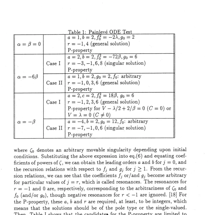
$\mathrm{F}\mathrm{i}_{\mathrm{o}}\sigma \mathrm{u}\mathrm{r}\mathrm{e}1$

shows the sections for the integrable

case

_{$\alpha=-6\beta$}

,

where

$\alpha=-2,$

$\beta=1/3,$

$\lambda=2$

and

$V=1/2$

are taken.

$\mathrm{F}\mathrm{i}_{\mathrm{o}}\sigma \mathrm{u}\mathrm{r}\mathrm{e}\mathrm{s}(\mathrm{a})$

and (b),

respectively, show the surfaces when

$\mathrm{E}=0.0072$

and

0.262. We can see that

the

closed smooth

curves are

$1.\mathrm{v}\mathrm{i}\mathrm{n}_{\mathrm{o}}\sigma$

on the surface even if the

energy

increases,

which means that the trajectories move on the tori in the

$\mathrm{o}\mathrm{r}\mathrm{i}_{\mathrm{o}}\sigma \mathrm{i}\mathrm{n}\mathrm{a}1$

phase

space

even

in the nonlinear

$\mathrm{r}\mathrm{e}_{\mathrm{o}}\sigma \mathrm{i}\mathrm{m}\mathrm{e}$

.

The

situation on the

$\mathrm{r}\mathrm{e}_{\mathrm{o}}\sigma \mathrm{u}\mathrm{l}\mathrm{a}\mathrm{r}$

motion of

the trajectories

is

similar when

$\alpha=-\beta$

,

if the

condition

_{$V-\lambda/2+2/\beta=0$}

is satisfied. Figure 2

shows this case, where

we

take

$\alpha=-4,$

$\beta=4,$

$\lambda=2$

and

$V=1/2$

.

As is

seen in both

$\mathrm{F}\mathrm{i}_{\mathrm{o}}\sigma \mathrm{s}.(\mathrm{a})$

for

$\mathrm{E}=0.0.36$

and (b)

for

$\mathrm{E}=0.216$

,

even

if the

energy

increases, the smooth

curves

are retained

on

the surface,

which

means that the motion of the trajectories is

.

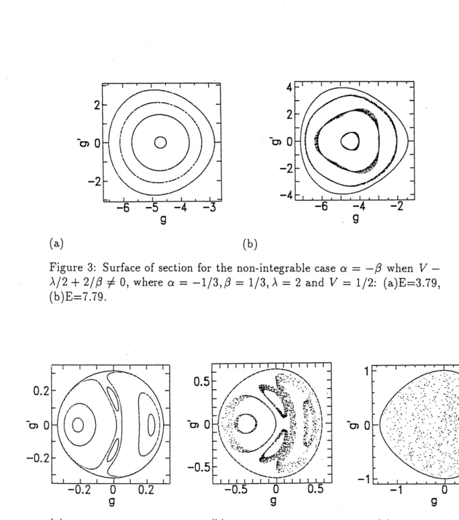
However, if this

condition is

not satisfied,

the motion of the trajectories are

$\mathrm{i}\mathrm{r}\mathrm{r}\mathrm{e}_{\mathrm{o}}\sigma \mathrm{u}\mathrm{l}\mathrm{a}\mathrm{r}$

in the

nonlinear

$\mathrm{r}\mathrm{e}_{\mathrm{o}}\sigma \mathrm{i}\mathrm{m}\mathrm{e}$

. This

is shown in Fig.3, where

$\alpha=-1/\cdot 3,$ $\beta=1/\cdot 3,$ $\lambda=2$

and

$V=1/‘ 2$ .

It

is found from both

Figs.(a)

for

$\mathrm{E}=3.79$

and

(b)

for

$\mathrm{E}=7.79$

that the smooth

curves are partly

replaced

by

$\mathrm{v}\mathrm{a}_{\mathrm{o}}\sigma \mathrm{u}\mathrm{e}\mathrm{l}\mathrm{y}$

scattered points, when

the

$\mathrm{e}\mathrm{n}\mathrm{e}\mathrm{r}_{\mathrm{O}}\sigma \mathrm{y}$

increases.

Furthermore,

in Fig.4

for

$\alpha=\beta$

,

we

can

illustrate one

of the examples which do

not

pass the test and show the large

regions

of

chaotic motion, where we take

$\alpha=\beta=1/\cdot 3,$ $\lambda=2$

and

$V=1/2$ .

$\mathrm{A}\mathrm{l}\mathrm{t}\mathrm{h}\mathrm{o}\mathrm{u}_{\mathrm{O}}\sigma \mathrm{h}$

closed smooth curves are

$1\mathrm{y}\mathrm{i}\mathrm{n}_{\mathrm{o}}\sigma$

on the surface for sufficiently

small

$\mathrm{e}\mathrm{n}\mathrm{e}\mathrm{r}_{\mathrm{o}}\sigma \mathrm{y}$

$\mathrm{E}=0.05(\mathrm{F}\mathrm{i}_{\mathrm{o}}\sigma.(\mathrm{a}))$

,

when the

energy

increases to

$\mathrm{E}=0.2(\mathrm{F}\mathrm{i}\mathrm{g}.(\mathrm{b}))$

,

the

curves

become

vague

due

to

scattering points

$\mathrm{a}\mathrm{l}\mathrm{o}\mathrm{n}_{\mathrm{o}}\sigma$

them. Finally, when

$\mathrm{E}=0.5$

,

all

smooth curves disappear and random

spread

of points are found all over the

surface within the maximum

energy

shell

$(\mathrm{F}\mathrm{i}_{\mathrm{o}}\sigma.(\mathrm{C}))$

.

(7)

(a)

(b)

$\mathrm{F}\mathrm{i}_{\mathrm{o}}^{\sigma \mathrm{u}\mathrm{r}\mathrm{e}}1$

:

Surface

of

section for

the

integrable case

$\alpha=-6\beta,$

$\mathrm{w}\mathrm{l}$

)

$\mathrm{e}\mathrm{r}\mathrm{e}\alpha=$

$-2,$

$\beta=1/3,$

$\lambda=2$

and

$V=1/2:(\mathrm{a})\mathrm{E}=0.0072,$

$(\mathrm{b})\mathrm{E}=0.262$

.

(a)

(b)

Figure

2:

Surface

of section for the

integrable

case

$\alpha=-\beta$

when

$V-$

$\lambda/2+2/\beta=0$

,

where

$\alpha=-4,$ $\beta=4,$

$\lambda=2$

and

$V=1/2$

:

(a)

$\mathrm{E}=0.0036$

,

(8)

(a)

(b)

Figure

3:

Surface of section for the non-integrable case

$\alpha=-\beta$

when

$V-$

$\lambda/2+2/\beta\neq 0$

,

where

$\alpha=-1/3,\beta=1/3,$

$\lambda=2$

and

_{$V=1/2:(\mathrm{a})\mathrm{E}=.3.79$}

,

$(\mathrm{b})\mathrm{E}=7.79$

.

(a)

(b)

(c)

Figure

4:

Surface

of

section

for the

non-integrable case

$\alpha=\beta$

,

where

$\alpha=$

(9)

3 Painlev\’e

PDE

test.

It

is known

that

the test in the

reduced ODE gives

only necessary conditions

for the

$\mathrm{o}\mathrm{r}\mathrm{i}_{\mathrm{o}}\sigma \mathrm{i}\mathrm{n}\mathrm{a}1$

PDE

to

be completely

.

$[16]$

In other words, a

$0\sigma \mathrm{i}\mathrm{v}\mathrm{e}\mathrm{n}$

PDE is not completel.V

when the

ODE

reduced from the

PDE

does

not have the

$\mathrm{P}$

-property.

Therefore,

in this

section,

the

of the

original PDE is directly examined for the three cases that pass the

ODE

test

in the

$\mathrm{p}\mathrm{r}\mathrm{e}\mathrm{C}\mathrm{e}\mathrm{d}\mathrm{i}\mathrm{n}_{\circ}\sigma$

section.

Let us apply the

Painlev\’e

_PDE

test,

whose direct procedure was

intro-duced by Weiss et al. [17] In this

test,

a

given partial

differential

equation

is

said

to

have the P- property if the solutions are

$\sin\sigma \mathrm{l}\mathrm{e}\mathrm{o}$

-valued

in the

neigh-borhood of the

arbitrary

and analytic (movable)

manifold.

Since

the

manifold for

the

ODE

reduces to the

$\sin_{\mathrm{O}}\sigma \mathrm{u}\mathrm{l}\mathrm{a}\mathrm{r}\mathrm{i}\mathrm{t}\mathrm{y}$

with respect

to

a

$\sin\sigma \mathrm{l}\mathrm{e}\mathrm{o}$

variable,

the

PDE

test may be

considered

as a

$\mathrm{s}\mathrm{t}\mathrm{r}\mathrm{a}\mathrm{i}_{\mathrm{o}}\sigma \mathrm{h}\mathrm{t}\mathrm{f}_{\mathrm{o}\mathrm{r}}\mathrm{w}\mathrm{a}\mathrm{r}\mathrm{d}$

extention of the

ODE

test

with similar procedure. For

convenience,

$\mathrm{r}\mathrm{e}\mathrm{w}\mathrm{r}\mathrm{i}\mathrm{t}\mathrm{i}\mathrm{n}_{\mathrm{o}}\sigma$

$\mathrm{e}\mathrm{q}.(4)$

in the followin\mbox{\boldmath $\sigma$}o form:

$\mathrm{i}n_{t}+u_{xx}=u\omega$

,

$-\mathrm{i}v_{t}+u_{xx}=vw$

,

$\omega_{t}+\alpha ww_{x}+\beta w_{xxx}=(uv)_{x}$

,

(10)

the solutions

are

set

as

$u= \phi^{-a}\sum_{j=0}u\infty j\varphi^{1j}$

,

$v= \phi^{-b}\sum_{j=0}v_{j}\phi^{j}\infty$

,

$w=( \delta^{-\mathrm{c}}\sum w_{j}\phi^{j}j=\infty 0^{\cdot}$

(11)

$\mathrm{M}\mathrm{a}\mathrm{k}\mathrm{i}\mathrm{n}_{\mathrm{O}}\sigma$

use of

(11)

into

$\mathrm{e}\mathrm{q}.(10)$

,

we can deterlnine the

$1\mathrm{e}\mathrm{a}\mathrm{d}\mathrm{i}\mathrm{n}_{\mathrm{o}}\sigma$

order

$a,$

$b$

and

$c$

and the

resonances

$r$

like

in the

ODE

test,

whose values are integers for the

same three cases of

$\alpha$

and

$\beta$

as

in Table I. The results of the PDE

test

are

shown

in Table II,

where

the

case

$\alpha=\beta=0$

have only

general

solution,

while

the other

two

cases have both

and

$0\sigma \mathrm{e}\mathrm{n}\mathrm{e}\mathrm{r}\mathrm{a}\mathrm{l}_{\mathrm{S}}\mathrm{o}\mathrm{I}\mathrm{u}\mathrm{t}\mathrm{i}\mathrm{o}\mathrm{n}\mathrm{S}$

.

$[19]\mathrm{C}\mathrm{h}\mathrm{e}\mathrm{c}\mathrm{k}\mathrm{i}\mathrm{n}_{\mathrm{o}}\sigma$

the

recursion relations for the self-consistency of the

resonances,

it is finally

found that the case of

$\alpha=\beta=0$

and the

Case

II

for

$\alpha=-\beta$

hold

the

$\mathrm{P}$

-property

without any

restrictions. The latter

case,

however,

is

excluded in

the present context,

since

the solutions

$u$

and

$v$

are

to

vanish closely

near

the

manifold

$\phi=0$

. Consequently, the

$\mathrm{s}\mathrm{i}_{\mathrm{o}}\sigma \mathrm{n}\mathrm{i}\mathrm{f}\mathrm{i}\mathrm{C}\mathrm{a}\mathrm{n}\mathrm{t}$

solution is

only

$w$

which

is

$\mathrm{n}\mathrm{o}\mathrm{t}\mathrm{h}\mathrm{i}\mathrm{n}_{\circ}\sigma$

but that

of the

K-dV equation,

where the

resonances

occur

for $r=-1,4,6$

.

On

the other

hand,

the other cases have

the

P-property

through the

$\mathrm{t}\mathrm{r}\mathrm{a}\mathrm{v}\mathrm{e}\mathrm{l}\mathrm{i}\mathrm{n}\circ\circ$

wave transformation like

$\phi=x-ct$

(

_$c$

:const.),

that

is

(10)

completely

,

which

is consistent with the result of

IST

method.

$[8, 9]$

4 Concluding

remarks.

We

can see in Table

II

that

the

leading orders and some coefficients in the

expansions are coincident or

adjustable

between the completely

$\mathrm{i}\mathrm{n}\mathrm{t}\mathrm{e}_{\mathrm{o}}\circ\cdot \mathrm{r}\mathrm{a}\mathrm{b}\mathrm{l}\mathrm{e}$

case

$\alpha=\beta=0$

and

the

case for

$\alpha=-6\beta$

(Case II).

Although this

$\mathrm{s}\mathrm{u}\mathrm{g}_{\mathit{0}}\sigma \mathrm{e}\mathrm{S}\mathrm{t}_{\mathrm{S}}$

that these

two

cases are

closely related to

each

other,

the

test

is found

not to

be successful in the nearly

$\mathrm{i}\mathrm{n}\mathrm{t}\mathrm{e}_{\mathrm{o}}\sigma \mathrm{r}\mathrm{a}\mathrm{b}\mathrm{l}\mathrm{e}\mathrm{r}\mathrm{e}_{\mathrm{o}}\sigma \mathrm{i}\mathrm{o}\mathrm{n}\alpha,$

$\beta\sim 0$

for

$\alpha=-6\beta$

,

since the

manifold

expansions become non-uniformly valid when

$\beta$

tends

to

zero. This

_{non-unifo,rmity}

may be due to the small parameter

$\beta$

in

the

$\mathrm{h}\mathrm{i}_{\mathrm{o}}\sigma \mathrm{h}\mathrm{e}\mathrm{S}\mathrm{t}$

order derivative term

in

. Additionally,

since

there

exists

one-soliton

solutions

which

are

uniformly

valid for

$\alpha=-6\beta \mathrm{i}\mathrm{n}\mathrm{C}\mathrm{l}\mathrm{u}\mathrm{d}\mathrm{i}\mathrm{n}_{\mathrm{o}}\sigma\alpha=\beta=0,$

$[10]$

the usual

manifold expansions

(9)

and

(11)

is not appropriate

to

examine the

in this region.

On

the other

hand,

in

the

$\circ\sigma \mathrm{e}\mathrm{n}\mathrm{e}\mathrm{r}\mathrm{a}\mathrm{l}$

solution for

$\alpha=-6\beta$

(Case II),

we

(11)

is

found

to

be

relaxed considerably for

a

finite time. That is

to

say,

since the

$\mathrm{s}\mathrm{i}_{\mathrm{o}}\sigma \mathrm{n}\mathrm{i}\mathrm{f}\mathrm{i}\mathrm{c}\mathrm{a}\mathrm{n}\mathrm{t}$

compatibility condition for the

$\mathrm{P}$

-property

is written as

$\theta_{t}-\theta\theta_{x}=0$

,

(12)

$\mathrm{t}\mathrm{h}\mathrm{r}\mathrm{o}\mathrm{u}_{\mathrm{o}}\sigma \mathrm{h}\theta=\phi_{t}/c)\mathcal{I}_{\text{ノ}}$

.

the

$0\sigma \mathrm{e}\mathrm{n}\mathrm{e}\mathrm{r}\mathrm{a}\mathrm{l}$

solution of the above wave

equ.ation

$\theta=(x \dagger t\theta)$

.

(13)

is

analytic

for a finite

time depending

upon initial conditions, where

$\ominus$

de-notes

an

arbitrary function. Therefore, for a

certain

class

of

$\acute{\varphi}$

which

is

given

by

(13)

$\mathrm{t}\mathrm{h}\mathrm{r}\mathrm{o}\mathrm{u}_{\mathrm{o}}\sigma \mathrm{h}\theta=\phi_{t}/\Phi_{x}’$

,

the

compatibility condition

(12)

can be

satisfied

for a finite time

$\mathrm{d}\mathrm{u}\mathrm{r}\mathrm{i}\mathrm{n}_{\mathrm{o}}\sigma$

which the solution

(13)

is analytic and arbitrary.

This means

that

the equation holds the

$\mathrm{P}$

-property

for

the finite time and is

expected

to

have multi-soliton solutions

for the

time. As

a

special

case,

it is

easil.v

seen that the condition

(12)

is

identically

satisfied for

an

infinitely

time under the

$\mathrm{t}\mathrm{r}\mathrm{a}\mathrm{Y}^{-}\mathrm{e}\mathrm{l}\mathrm{i}\mathrm{n}_{\mathrm{o}}\sigma$

wave

transformation

$\mathit{0}’=x-ct$

,

which

is

confirmed

by

the

existence of one-soliton solution. [10]

Thus,

for

$\alpha=-6\beta,$

$\mathrm{t}\mathrm{h}\mathrm{o}\mathrm{u}_{\mathrm{o}}\sigma \mathrm{h}$

one

soliton

state

is valid for an infinitely

time.,

the soliton

interactions

due

to

multi-soliton state

$\mathrm{n}\dot{\mathrm{u}}_{\mathrm{o}}\sigma \mathrm{h}\mathrm{t}$

be elastic

for

the

finite

time,

that

is

to say, the

possibility of

’finite time

’

is expected.

References

[1]

D.J. Benney, Stud.

Appl.Math.55 (1976)93.

[2]

A.D.D.Craik.

PVaue interactions and

_{fiuid fiows}

(

$\mathrm{C}\mathrm{a}\mathrm{m}\mathrm{b}\mathrm{r}\mathrm{i}\mathrm{d}_{\mathrm{o}}\sigma \mathrm{e}$

University

Press,

1985).

[3]

G.D.Crapper.

Introduction to water waves

(Ellis

Horwood,

1984).

[4] V.E.Zakharov, Sov.Phys.35(1972)908,

and see also

Sov.

J. Eksp.Theor.

Phys.62(1972)1745.

[5]

$\perp l\mathrm{I}.\mathrm{V}$

.

Goldman,

Rev.

Mod.Phys.56(1984)709.

(12)

[7]

$\mathrm{T}.\mathrm{Y}_{\mathrm{o}\mathrm{S}}\mathrm{h}\mathrm{i}\mathrm{n}\mathrm{a}\mathrm{o}\sigma \mathrm{a}$

,

M.Wakamiya and

T.Kakutani,

Phys.Fluids

_{$\mathrm{A}3(1991)8.3$}

,

and

see

also

$\mathrm{T}.\mathrm{Y}_{0}\mathrm{s}\mathrm{h}\mathrm{i}\mathrm{n}\mathrm{a}\sigma \mathrm{a}\mathrm{o}$

and

T.Kakutani,

J.Phys.Soc..Jpn.

63 (1994)445

and the

references therein.

[8]

N.Yajima and M.Oikawa,

$\mathrm{P}\mathrm{r}\mathrm{o}^{\sigma}.\mathrm{T}\mathrm{o}\mathrm{y}\mathrm{h}\mathrm{e}\mathrm{o}\mathrm{r}.\mathrm{P}\mathrm{h}\mathrm{s}.56(1976)1719$

.

[9]

Y-C.Ma,

Stud.

in

Appl.Math.59(1978)201.

[10]

$\mathrm{T}.\mathrm{Y}^{r}\mathrm{o}\mathrm{S}\mathrm{h}\mathrm{i}\mathrm{n}\mathrm{a}\sigma \mathrm{a}\circ$

and T.Kakutani, J.Phys.Soc.Jpn.63(1994)445.

[11]

E.S.Benilov and

S.P.Burtsev, Phys.Lett.

$\mathrm{A}98(198.3)256$

.

[12]

$\mathrm{T}.\mathrm{Y}_{\mathrm{o}\mathrm{S}}\mathrm{h}\mathrm{i}\mathrm{n}\mathrm{a}_{\mathrm{o}}\sigma \mathrm{a}$

,

Proc.Estonian Acad.Sci.Phys.Math.,44

(1995)

96. [1.3]

M.Tabor,

Chaos

and

integrability

in

nonlinear

dynamics

(John

Wiley&

Sons,

New

York, 1989).

[14]

M.J.Ablowitz

and P.A.Clarkson,

Solitons,

Nonlinear Evolution

Equa-tions and Inverse

Scattering

(London Vl

Iathematical Society Lecture

Note

Series

$149,\mathrm{C}\mathrm{a}\mathrm{m}\mathrm{b}\mathrm{r}\mathrm{i}\mathrm{d}_{\mathrm{o}}\sigma \mathrm{e}$

Univ.Press,

$\mathrm{C}^{\mathrm{t}}\mathrm{a}\mathrm{m}\mathrm{b}\mathrm{r}\mathrm{i}\mathrm{d}\mathrm{o}\sigma \mathrm{e}$

,

1991).

[15]

$\mathrm{Y}.\mathrm{F}.\mathrm{C}\mathrm{h}\mathrm{a}\mathrm{n}_{\mathrm{o}}\sigma$

,

M.Tabor and J.Weiss,

J.Math.Phys.23(1982)531.

[16] M.J.Ablowitz,

A.Ramani and

$\mathrm{H}.\mathrm{S}\mathrm{e}_{\mathrm{o}}\sigma \mathrm{u}\mathrm{r}$

,

J.Math.Phys.21

(1980)

715.

$[17].].\mathrm{t}\mathrm{V}\mathrm{e}\mathrm{i}_{\mathrm{S}\mathrm{s}}$

,

M.Tabor and G.Carnevale,

J.Math.Phys.24(1983)

522. [18] R.Conte, A.P.Fordy and A.

$\mathrm{P}\mathrm{i}\mathrm{c}\mathrm{k}\mathrm{e}\mathrm{r}\mathrm{i}\mathrm{n}_{\mathrm{o}}\sigma$

,

Physica D69

(1993)33

and

the

references therein.

[19] T.

$\mathrm{Y}\mathrm{o}\mathrm{s}\mathrm{h}\mathrm{i}\mathrm{n}\mathrm{a}\sigma \mathrm{a}\mathrm{o}$