The quantities W, L, K and variations of
geodesics in Finsler spaces
Tetsuya NAGANO
Abstract
The author investigates the first and the second variations of the arc length of curves under the standpoint of linear parallel displacements. Last year the author studied linear parallel displacements along an infinitesimal parallelogram and
ob-tained three quantities on H([9],[10]). In this paper, they appear in the second
variation.
Keywords and phrases : linear parallel displacement, first variation, second vari-ation, locally Minkowski space, Finsler geometry.
Introduction
The author have been studying the linear parallel displacement in Finsler geometry from 2008. In [4] the author called it “parallel displacement”. But in [6] and [7] the author renamed it “linear parallel displacement” because Prof.Z.Shen had already given the nearly same definition satisfying the linearity by the coefficients Ni
j in his book [1] .
He called such parallel displacements “linear parallel”.
First, we put terminology and notations used in this paper(cf.[2] and [3]). Let M be an n-dimensional differentiable manifold and x = (xi) a local coordinate of M . T M is the
tangent bundle of M and (x, y) = (xi, yi) is a local coordinate of T M . N = (Ni j(x, y))
is an non-linear connection of T M and its coefficients of N on a local coordinate (x, y).
F (x, y) is a Finsler structure (or Finsler metric, Finsler fundamental function) on M .
Further, F Γ = (Ni
j(x, y), Fjri (x, y), Cjri (x, y)) is Finsler connection and its coefficients
of F Γ satisfying Trji := Frji − Fjrr = 0, Dji := yrFrji − Nji = 0 and gij|k(x, y) = 0(h-metrical). And Ni
j(x, y), Fjki (x, y), Crji (x, y) are positively homogeneous of degree 1, 0
and –1, respectively. Therefore Ni
j and Fjri come to Cartan’s ones. Last, we denote the
collection of horizontal vectors at every point on T M byH. This is the subbundle of T T M and its dimension is 3n. So we denote a local coordinate ofH by (x, y, z). And it is called “horizontal subbundle of T T M ”. All of objects appeared in this paper (curves, vector fields, etc) are differentiable. In additions, indexes a, b, c,· · · , h, i, j, k, l, m, · · · , α, β, · · · , run on from 1 to n = dimM .
Now, for a vector field on a curve c with a parameter t, we give a following definition of linear parallel displacements along c([4],[5],[6],[7]).
Definition 0.1 For a curve c = (ci(t)) (a≤ t ≤ b) on M and a vector field v = (vi(t))
along c, if the equation
(0.1) dv i dt + v jFi jr(c, ˙c) ˙c r= 0 ( ˙cr = dcr dt )
is satisfied, then v is called a parallel vector field along c, and we call the linear map
Πc: v(a) −→ v(b) a linear parallel displacement along c.
The difference from the traditional notion of parallel displacement in Finsler geometry are three points. One of them is that the inverse vector field v−1(τ )(τ = −t + α) is not always parallel along the inverse curve c−1(τ ), even if v(t) is parallel vector field along a curve c(t)(cf.[4], [6]).
The others of them are that we can consider, for vector fields u(t), v(t) along c(t), an inner product gij(c, ˙c)ui(t)vj(t) along the curve c(t) and the inner product is not always
preserved, even if u, v are parallel vector fields along a curve c. Then we have(cf.[5])
Proposition 0.1 Let (M, F (x, y)) be a Finsler space with a Finsler connection (Ni
j, Fjri , Cjri )
satisfying h-metrical gij|r = 0. For any parallel vector fields v = (vi(t)), u = (ui(t)) along
a curve c = (ci(t)), if c is a path or a geodesic, then the inner product gij(c, ˙c)viuj along
c is preserved.
Theorem 0.1 Let (M, F (x, y)) be a Finsler space with a Finsler connection. We
assume that the Finsler connection is h-metrical and the metric gij is positive definite.
Any smooth curve preserves the inner products of parallel vector fields along it, if and only if, ∂gij
∂yr = 0 is satisfied, namely, (M, gij) is a Riemannian space.
1
Linear parallel displacements along an infinitesimal
parallelogram
Next we introduce conclusions obtained by investigating linear parallel displacements along an infinitesimal parallelogram([9],[10]).
We studied two cases. One is the case that makes an initial vector be two parallel vector fields along two routes(Case I), and the other is the case making a parallel vector field along one loop(Case II). Hereafter, we assume all points and curves are in one coordinate neighborhood.
First, we define three quantities W, L, K onH as follows:
Whji (x, y, z) := Fhji (x, y)− Fhji (x, z), (1.1) Lihj(x, y, z) := ∂F i hm ∂yj (x, y)z m+∂Fhmi ∂zj (x, z)y m, (1.2) Khjki (x, y, z) := δF i hj δxk (x, y)− δFi hk δxj (x, z)− F i mj(x, y)F m hk(x, y) + F i mk(x, z)F m hj(x, z). (1.3)
Case I. Let p, q, r, s be four points on M and let (xi), (xi+ ξi), (xi+ ξi+ ηi), (xi+ ηi) be their coordinates, respectively. Further c1, c2, c3, and c4 are following curves with a
parameter t (0≤ t ≤ 1): (I) c1(t) : xi(t) = xi+ tξi (p to q), c2(t) : xi(t) = xi+ ξi+ tηi (q to r), c3(t) : xi(t) = xi+ tηi (p to s), c4(t) : xi(t) = xi+ ηi+ tξi (s to r).
We take two routes c = c1+ c2(p → q → r) and ¯c = c3 + c4(p → s → r), and consider
linear parallel displacements along c and ¯c, respectively. Let V = (Vi) be an initial vector
at p and let Vq, Vrbe the values at q and r by the parallel vector field along c, respectively.
Further, let ¯Vs, ¯Vr the value at s and r by the parallel vector field along ¯c, respectively.
Our standpoint is to investigate the difference ¯Vr− Vr. The result is as follows:
¯
Vri− Vri = [Whji (x, ξ, η)(ξj + ηj) + Lhji (x, ξ, η)(ηk− ξk) + Khjki (x, ξ, η)ηjξk]Vh+· · · . (1.4)
Case II. Let four points p, q, r, s be the same in Case I. However, curves c3, c4 are
different from (I) as follows
(II) c1(t) : xi(t) = xi + tξi (p to q), c2(t) : xi(t) = xi + ξi+ tηi (q to r), c3(t) : xi(t) = xi + ξi+ ηi− tξi (r to s), c4(t) : xi(t) = xi + η− tηi (s to p), where 0≤ t ≤ 1.
We take a loop c = c1 + c2 + c3 + c4(p → q → r → s → p) and consider a linear
parallel displacement along c. Let V = (Vi) be an initial vector at p and let V
q, Vr, Vs be
the values of the parallel vector field along c at q, r, s, respectively. Further, let ¯V be the
value at the end point p.
Our standpoint is to investigate the difference ¯V − V . The result is as follows:
¯
Vi− Vi
= [Whji (x,−η, ξ)(ξj + ηj) + Lihj(x,−η, ξ)(ηj − ξj) + Khjki (x,−η, ξ)ξjηk]Vh+· · · . (1.5)
Remark 1.1 In (1.4) and (1.5), (· · · ) expresses 3rd and more order terms with respect
to ξ, η.
After all, we have the following theorem([9],[10]).
Theorem 1.1 Let M be an n-dimensional differentiable manifold with a Finsler
con-nection F Γ = (Ni
j(x, y), Fjki (x, y), Cjki (x, y)) satisfying Tjki (x, y) = 0, Dji(x, y) = 0. First,
for an infinitesimal parallelogram defined by (I) and an initial vector V = (Vi), we have
the difference ¯Vr − Vr satisfying (1.4). Next, for an infinitesimal parallelogram defined
by (II) and an initial vector V = (Vi), the parallel vector ¯V = ( ¯Vi) is obtained and the
differences ¯V − V satisfies (1.5).
After that the author studied in detail properties of W, L, K in [10] and obtained the following propositions and theorem.
Proposition 1.1 (Proposition 3.1 in [10]) Let F Γ = (Nji(x, y), fhji (x, y), Chji (x, y)) be
a Finsler connection satisfying Ti
rj = 0 and Dji = 0. Then W = 0 on H is equivalent to
Proof
From Wi
hj(x, y, z) = 0, Fhji (x, y) = Fhji (x, z) is satisfied. This implies
(1.6) ∂F i hj ∂yk (x, y) = ∂Fhji ∂zk (x, z) = 0. Therefore Li hj(x, y, z) = 0 is satisfied.
Inversely, we assume Lihj(x, y, z) = 0. Then the following equation
(1.7) ∂F i hm ∂yj (x, y)z m =−∂Fhmi ∂zj (x, z)y m
is satisfied on any points (x, y, z). We take partial derivations by yl and zk of both sides,
respectively. Then we have
(1.8) ∂ 2Fi hk ∂yj∂yl(x, y) =− ∂2Fi hl ∂zj∂zk(x, z).
This means that the derivative of the second order by the second variable of the coefficient
Fi
hj has no the second variable. Namely,
(1.9) ∂F i hj ∂yk (x, y) = Q i hjkm(x)y m is satisfied.
On the other hand, Fhji (x, y) is positively homogeneous of degree 0 with respect to the variable y. So ∂F
i hj
∂yk (x, y)y
k = 0 is satisfied. Therefore we have
(1.10) Qihjkm(x)ymyk= 0.
The above quadratic form of y is satisfied on any y so Qihjkm(x) = 0 must be true. Therefore we have ∂F i hj ∂yk (x, y) = 0. Namely, (1.11) Whji (x, y, z) = 0 is satisfied. Q.E.D.
In addition, according to the above proof, we have the following proposition.
Proposition 1.2 (Proposition 3.2 in [10]) Let F Γ = (Ni
j(x, y), fhji (x, y), Chji (x, y)) be
a Finsler connection satisfying Trji = 0 and Dji = 0. If W = 0 is satisfied on H, then
∂Fi hj
∂yk (x, y) = 0, namely, F
i
hj = Fhki (x) is satisfied on T M .
Further, if we assume Whji (x, y, z) = 0 and Khjki (x, y, z) = 0 on H, then we can prove the following proposition.
Proposition 1.3 (Proposition 3.3 in [10]) Let F Γ = (Ni
j(x, y), fhji (x, y), Chji (x, y))
be a Finsler connection satisfying Ti
rj = 0 and Dji = 0. For any point (x, y, z) on H,
if Whji (x, y, z) = 0 and Khjki (x, y, z) = 0 are satisfied, then the torsion tensor fields
Pi
hj(x, y), Rihj(x, y), Chji (x, y) and the curvature tensor fields Rihjk(x, y), Phjki (x, y) of F Γ
satisfy the following equations:
(1.12) Phji (x, y) = 0, Rihj(x, y) = 0, Phjki (x, y) + Chki |j(x, y) = 0, Rihjk(x, y) = 0.
Proof
Since Proposition 1.2, ∂F
i hj
∂yk (x, y) = 0 is satisfied. From Phji =
∂Ni h ∂yj − Fjhi and Nji = ymFi mj(D = 0), (1.13) Phji (x, y) = 0 is satisfied. Next, from ∂F
i hj ∂yk = Phjki + Chki |j− Chqi P q jk and P i hj = 0, we have (1.14) Phjki (x, y) + Chki |j(x, y) = 0.
And from Khjki (x, y, z) = 0, of course Khjki (x, y, y) = 0 is satisfied. In addition, in general, Ki
hjk(x, y, y) = Rihjk(x, y)− Chmi (x, y)Rjkm(x, y) is true. So Rhjki − Chmi Rmjk = 0 is
satisfied. And from Ri
jk = ym(Rimjk− Cmsi Rsjk), we have
(1.15) Rijk(x, y) = 0. We apply the above conclusion in Ri
hjk− Chmi Rmjk = 0 again, then we obtain
(1.16) Rhjki (x, y) = 0.
Q.E.D.
For a Finsler space, the author stated in detail the conditions to be locally Minkowski space in [8]. If we apply Proposition 1.3 to the Finsler space with the property of h-metrical, then we have the following theorem.
Theorem 1.2 (Theorem 3.2 in [10]) Let (M, F, F Γ) be a Finsler space with the Finsler
connection F Γ = (Ni
j(x, y), Fjki (x, y), Cjki (x, y)) satisfying Tjki = 0, Dji = 0 and gij|k = 0.
If W and K vanish on H, then the Finsler space (M, F, F Γ) is a locally Minkowski space and the inverse property is also true.
2
The first and the second variations of arc lengths
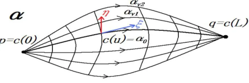
Now we investigate the first and the second variations of arc lengths under the stand-point of linear parallel displacements. Let p, q be stand-points on M and let c(u) (u: arc length, 0 ≤ u ≤ L) be a curve from p to q. I is an open interval including the closed interval [0, L], where p = c(0), q = c(L). Further Iϵ = (−ϵ, ϵ) is an infinitesimal open interval.
Then a variation α(u, v) is a differentiable map as follows:
where α(u, 0) = c(u). Then αv(u) := α(u, v) with fixed v is called “variational curve”.
Further we denote vector fields ∂α∂u = ∂x∂ui∂x∂i and
∂α ∂v = ∂xi ∂v ∂ ∂xi by ξ and η, respectively.
Namely, we put ξ = ∂α∂u and η = ∂α∂v. Especially, η is called “variational vector”. In addition, we denote the coefficients of ξ and η by ξi := ∂xi
∂u and η
i := ∂xi
∂v, respectively.
First, from ∂u∂v∂2xi = ∂v∂u∂2xi we have very important relation as follows:
(2.2) ∂ξ
i
∂v = ∂ηi
∂u.
And on the curve c, we also have the following equations
(2.3) ξ = ˙c = dc
du, F (c, ˙c) =
√
gij(x, ˙c) ˙ci˙cj = 1.
In addition, we use following notations (2.4)
< ξ, ξ >ξ:=∥ ξ ∥2ξ= gij(x, ξ)ξiξj, < η, η >ξ:=∥ η ∥2ξ= gij(x, ξ)ηiηj, < ξ, η >ξ:= gij(x, ξ)ξiηj.
From (2.3) and (2.4), on c, we have
(2.5) < ˙c, ˙c >˙c=∥ ˙c ∥2˙c= 1.
We assume that variation α(u, v) keeps the endpoints p, q fixed. Then variational vector η(0, v) = η(L, v) = o are satisfied(See Figure 1). Here we put L(v) as the arc length of a variational curve αv as follows:
(2.6) L(v) = ∫ L 0 F (α,∂α ∂u)du = ∫ L 0 √ gij(x, ξ)ξiξjdu.
Here we put the following definition.
Definition 2.1 The quantity L′(0) = dLdv|v=0 is called “first variation” of L(v) with
respect to the variation α and the curve c which satisfies L′(0) = 0 is called “extremal(or
critical) curve”.
Figure 1: Variation
We consider the following variational problems: 1. Find extremal curve out!
For the above Problem 1, we need (2.7) L′(v) = ∫ L 0 F′du = ∫ L 0 ∂F ∂vdu.
If we use, for (2.7), the following formations (2.8)∼ (2.13):
F′ = ∂F ∂xi ∂xi ∂v + ∂F ∂ξi ∂ξi ∂v = ∂F ∂xiη i+ ∂F ∂ξi ∂ηi ∂u, (2.8) ∂gλµ ∂yi (x, ξ)ξ λ ξµ= 0, (2.9) ∂F ∂xi = 1 2F ∂F2 ∂xi = 1 2F ∂ ∂xi(gλµ(x, ξ)ξ λξµ) = 1 2F ∂gλµ ∂xi (x, ξ)ξ λξµ, (2.10) ∂F ∂ξi = 1 2F ∂F2 ∂ξi = 1 2F ∂ ∂ξi(gλµ(x, ξ)ξ λξµ) = 1 2F( ∂gλµ ∂yi (x, ξ)ξ λξµ+ 2ξ i) = 1 Fξi, (2.11) ∇ξηi := ∂ηi ∂u + F i αβ(x, ξ)ξ α ηβ, (2.12) ξi = gij(x, ξ)ξj, gij|r = 0. (2.13)
then we can obtain
(2.14) F′ = 1 Fξi∇ξη i. From F′ = F1ξi∇ξηi = F1gij(x, ξ)ξj∇ξηi = F1 < ξ,∇ξη >ξ, we obtain (2.15) L′(v) = ∫ L 0 1 F < ξ,∇ξη >ξ du,
and, on curve c, from v = 0, F = 1 and ξ = ˙c, we have
(2.16) L′(0) = ∫ L
0
< ˙c,∇˙cη >˙c du.
In addition, from gij|k = 0 and ∂gij
∂yk(c, ˙c) ˙c
i = 0, we have d
du < ˙c, η >˙c=< ∇˙c˙c, η >˙c + <
˙c,∇˙cη >˙c. Therefore we can have
(2.17) L′(0) =< ˙c, η >˙c |L0 −
∫ L
0
<∇˙c˙c, η >˙c du.
At the end point, η(0, v) = η(L, v) = o are true. After all, we can obtain
(2.18) L′(0) =− ∫ L
0
<∇˙c˙c, η >˙cdu.
Therefore the following proposition is true.
Theorem 2.1 Geodesic(∇˙c˙c = 0) is an extremal curve. Inversely, for any variation
Next, let’s investigate Problem 2. We must calculate the following expression.
(2.19) L′′(v) = ∫ L
0
F′′du.
If we use, for (2.19), the following formations (2.20)∼ (2.23):
F′ = 1 Fgij(x, ξ)ξ j∇ ξηi, F′′ = ∂ ∂v( 1 Fgij(x, ξ)ξ j∇ ξηi), (2.20) ∇ηξµ = ∂ξµ ∂v + F µ αβ(x, η)η αξβ, ∇ ξηµ= ∂ηµ ∂u + F µ αβ(x, ξ)ξ αηβ, (2.21) ∂ξµ ∂v = ∂ηµ ∂u , ∇ξη µ=∇ ηξµ+ Wαβµ (x, ξ, η)ξ αηβ, (2.22) ∇η∇ξηλ = ∂ ∂v(∇ξη λ) + Fλ αβ(x, η)η α∇ ξηβ, ξα = gδα(x, ξ)ξδ, gij|k = 0, (2.23)
then we can obtain (2.24) F′′ = 1 Fξλ∇η∇ξη λ+ (1 Fgλµ(x, ξ)− 1 F3ξλξµ)∇ξη µ∇ ξηλ+ Ψβληβ∇ξηλ, where Ψβλ = F1(Fβλα(x, ξ)− F α βλ(x, η))ξα = F1Wβλα(x, ξ, η)ξα(̸= 0).
On the curve c, v = 0, F = 1 and ξ = ˙c are true. So we have
(2.25) F′′=< ˙c,∇η∇˙cη >˙c +∥ ∇˙cY ∥2˙c − < ˙c, ∇˙cη >2˙c + < ˙c, w >˙c,
where w = (Wα
βλ(c, ˙c, η)ηβ∇˙cηλ).
Here, we need the following formation to arrange < ˙c,∇η∇˙cη >˙c,
∇η∇˙cηk− ∇˙c∇ηηk.
According to linear parallel displacements along the infinitesimal parallelogram, we have the following formation
∇η∇˙cηk− ∇˙c∇ηηk= Whjk(c, η, ˙c)(η j + ˙cj)ηh+ Lk hj(c, η, ˙c)( ˙c j − ηj)ηh+ Kk hrj(c, η, ˙c) ˙c rηjηh. (2.26)
Let consider two parallel vector fields η −→ Π˙cη −→ ΠηΠ˙cη and η −→ Πηη −→
Π˙cΠηη along an infinitesimal parallelogram. Then the difference ΠηΠ˙cη− Π˙cΠηη is
ex-pressed as follows: ΠηΠ˙cη− Π˙cΠηη
= [Whjk(c, η, ˙c)(ηj + ˙cj) + Lkhj(c, η, ˙c)( ˙cj − ηj) + Khrjk (c, η, ˙c) ˙crηj]ηh+· · · . Now we denote by rk the difference ∇
η∇˙cηk − ∇˙c∇ηηk in (2.26). Then, from <
˙c,∇η∇˙cη >˙c=< ˙c,∇˙c∇ηη >˙c + < ˙c, r >˙c, (2.25) turns into the following formation
(2.27) F′′=< ˙c,∇˙c∇ηη >˙c +∥ ∇˙cη∥2˙c − < ˙c, ∇˙cη >2˙c + < ˙c, r + w >˙c . Then we have (2.28) L′′(0) = ∫ L 0 { < ˙c,∇˙c∇ηη >˙c +∥ ∇˙cη ∥2˙c − < ˙c, ∇˙cη >2˙c + < ˙c, r + w >˙c } du.
Definition 2.2 The quantity L′′(0) in (2.28) is called “second variation” of L(v) with
respect to the variation α.
Furthermore, from dud < ˙c,∇ηη >˙c=< ∇˙c˙c,∇ηη >˙c + < ˙c,∇˙c∇ηη >˙c, we have
(2.29)
F′′ = d
du < ˙c,∇ηη >˙c − < ∇˙c˙c,∇ηη >˙c+∥ ∇˙cη∥
2
˙c − < ˙c, ∇˙cη >2˙c + < ˙c, r + w >˙c.
Therefore we can obtain (2.30) L′′(0) =< ˙c,∇ηη >˙c|L0− ∫ L 0 <∇˙c˙c,∇ηη >˙c du+ ∫ L 0 { ∥ ∇˙cη∥2˙c − < ˙c, ∇˙cη >2˙c + < ˙c, r + w >˙c } du.
Here we add an assumption “c is geodesic”, then we have
(2.31) L′′(0) = ∫ L 0 { ∥ ∇˙cη∥2˙c − < ˙c, ∇˙cη >2˙c + < ˙c, R( ˙c, η) >˙c } du, R( ˙c, η) := r + w.
Furthermore, if Z := η− < ˙c, η >˙c ˙c, from < ˙c, Z >˙c= 0, then∇˙cZ =∇˙cη− < ˙c, ∇˙cη >˙c ˙c
and ∥ ∇˙cZ ∥2˙c=∥ ∇˙cη ∥2˙c − < ˙c, ∇˙cη >2˙c are satisfied. After all we obtain
(2.32) L′′(0) = ∫ L 0 { ∥ ∇˙cZ ∥2˙c + < ˙c, R( ˙c, η) >˙c } du, and (2.33) Rk( ˙c, η) = Whjk(c, η, ˙c)ηh(ηj+ ˙cj−∇˙cηj)+Lhjk (c, η, ˙c)ηh( ˙cj−ηj)+Khrjk (c, η, ˙c)ηh˙crηj. Then we have
Theorem 2.2 Let α(u, v) be a variation that the curve c is a geodesic. Then the
second variation L′′(0) satisfies the equation (2.32) with R( ˙c, η) of (2.33).
Theorem 2.3 We assume (2.32) and (2.33). Then
1. If the space is Riemannian, then R consists of Riemannian curvature Kαβik (c) only,
namely, Rk = Kk
αβi(c)ηα˙cβηi.
2. If the space is locally Minkowski, then R≡ 0 is satisfied.
3. The set of spaces which satisfy R≡ 0 involves Riemannian spaces and locally Minkowski
spaces.
Remark 2.1 If we use ∇ηξµ = ∂ξ
µ
∂v + F
µ
αβ(x, ξ)ηαξβ(usual manner), then R leads us
to the well-known flag curvature.
Next we put the following definition.
Definition 2.3 We call the quantity−< ˙c,R( ˙c,η)>c˙
∥Z∥2 ˙
c
“sectional curvature” with respect to
˙c and η at point c, and we denote it by ρ( ˙c, η)˙c. Namely,
(2.34) ρ( ˙c, η)˙c =−
< ˙c, R( ˙c, η) >˙c
∥ Z ∥2 ˙c
where if Z = o, then ρ( ˙c, η)˙c = 0. Then the second variation is modified to (2.35) L′′(0) = ∫ L 0 { ∥ ∇˙cZ ∥2˙c − ∥ Z ∥ 2 ˙c ρ( ˙c, η)˙c } du.
In Riemannian geometry, there is the notion of “relatively minimal curve”. So we put the notion in Finsler geometry as follows:
Definition 2.4 For any variation of a curve c, which keeps endpoints fixed, if the arc
length of c is always minimal for those of all variational curves, then c is called “relatively minimal curve” with respect to the endpoints.
“We assume that variations have the property which its variational vector field on the curve c is linearly independent to the tangent vector field ˙c of c at least one point.”
Then we have
Theorem 2.4 If ρ( ˙c, η)˙c ≤ 0 is satisfied on M, then any geodesic c is relatively
min-imal curve with respect to any endpoints on it.
Proof
We prove this property by a reduction to absurdity.
At first, from (2.35), we notice L′′(0)≥ 0, ∥ ∇˙cZ ∥2˙c≥ 0 and − ∥ Z ∥2˙c ρ( ˙c, η)˙c ≥ 0.
If L′′(0) = 0 is satisfied, then we have ∥ ∇˙cZ ∥2˙c= 0 and − ∥ Z ∥2˙c ρ( ˙c, η)˙c = 0. From
∥ ∇˙cZ ∥2˙c= 0,
(2.36) ∇˙cZ = 0
is satisfied. We notice that Z is a parallel vector field along c in the sense of linear parallel displacements from (2.36), and c is a geodesic. Therefore its norm ∥ Z ∥˙c is constant on
c. At a start point, η = 0 is satisfied, so ∥ Z ∥˙c= 0 holds good on c. Therefore Z is zero
vector field on c. Then
(2.37) η =< ˙c, η >˙c ˙c
is satisfied. Our assumption, however, can not permit (2.37) because Z and ˙c are linearly independent at least one point on c.
Therefore
(2.38) L′′(0) > 0 is satisfied.
This conclusion means that the geodesic c is minimal.
References
[1] S.-S. Chern and Z. Shen. Riemann-Finsler geometry, volume 6 of Nankai Tracts in
Mathematics. World Scientific Publishing Co. Pte. Ltd., Hackensack, NJ, 2005.
[2] M. Matsumoto. Foundations of Finsler geometry and special Finsler spaces. Kaiseisha Press, Shigaken, 1986.
[3] M. Matsumoto. Finsler geometry in the 20th-century. In Handbook of Finsler
geom-etry. Vol. 1, 2, pages 557–966. Kluwer Acad. Publ., Dordrecht, 2003.
[4] T. Nagano. Notes on the notion of the parallel displacement in Finsler geometry.
Tensor (N.S.), 70(3):302–310, 2008.
[5] T. Nagano. On the parallel displacement and parallel vector fields in Finsler geometry.
Acta Math. Acad. Paedagog. Nyh´azi., 26(2):349–358, 2010.
[6] T. Nagano. A note on linear parallel displacements in Finsler geometry. Journal of
the Faculty of Global Communication, University of Nagasaki, 12:195–205, 2011.
[7] T. Nagano. On the conditions for Finsler spaces to be locally flat Riemannian spaces.
preprint, 2011.
[8] T. Nagano. On the conditions to be locally Minkowski spaces. Proceedings of the
Conference RIGA 2011, pages 209–216, 2011.
[9] T. Nagano. The quantities derived from linear parallel displacements along an in-finitesimal parallelogram. Journal of the Faculty of Global Communication,
Univer-sity of Nagasaki, 13:129–141, 2012.
[10] T. Nagano. On the quantities W, L, K derived from linear parallel displacements in Finsler geometry. Journal of the Faculty of Global Communication, University of
Nagasaki, 14:123–132, 2013.
Department of Information and Media Studies University of Nagasaki