なぜ今GLMMなのか
竹澤正哲
北海道大学
日本社会心理学会第
2回春の方法論セミナー
院生時代、あるデータに出会った
「よし、条件は被験者内要因だから
反復測定ロジスティック回帰をしよう」
実験者
のカード
自分の
カード
条件
1
交換する
or
交換しない
⇒ ・・・
実験者
のカード
自分の
カード
条件
2
交換する
or
交換しない
⇒
実験者
のカード
自分の
カード
条件
3
交換する
or
交換しない
⇒
実験者
のカード
自分の
カード
条件
4
交換する
or
交換しない
⇒
• SASもSPSSも、どこを探しても、反復測定ロジスティック回
帰なんて見当たらない
• 大津起夫先生(現大学入試センター)
「一般推定方程式モデル(Generalized Estimation
Equation model)で分析すればいい。SASのproc genmod
でできるから」
• 後から分かったが、これはGLMMの親戚だった→ここから
私とGLMMとの出会いが始まる
一般化線形混合モデル
•
2000年代に生態学を中心として利用され始める
• 同時期、沓掛展之氏(総研大)、久保拓弥氏(北大)が
相次いで、インターネット上で情報を提供し始める
•
Bolker et al. (2009). Generalized linear mixed model: A
prac>cal guide for ecology and evolu>on. Trends in
Ecology and Evolu2on. doi:10.1016/j.tree.2008.10.008
ü 個人的にオススメ。 被引用回数は2000に迫る
• 久保拓弥(2012)「データ解析のための統計モデリング
何が凄いって…
GLMMの場合
分散分析、重回帰分析、ロジスティック回帰、多項ロジット、
対数線形モデル
…などが1つでできる
• 鍵となるのが、確率分布とリンク関数という2つの概念
• この2つをオプションとして指定することで、多様なデータを1
つのモデル内で分析できる
独立変数:
カテゴリカル/連続変量
従属変数:
連続変量(正規分布)
一般線形モデル(分散分析+重回帰分析)の場合
それぞれ無関係だと考えて来た人も多いのでは?
• 同一の参加者から繰り返しデータが測定されたら
• 反復測定分散分析
• 複数の集団が存在し、個人はその集団のどれかに
所属していたら
• 階層線形モデル(マルチレベルモデル)
• 枝分かれ実験のように条件がネストしていたら
• 平均平方和と自由度をあれこれいじって…
• は、反復測定?
変量効果(
random effects)というたった1つの概念
で、全てを扱えることを知っていましたか?
変量効果(Random Effects)
• 反復測定=被験者内要因
y
ij
= 個人 i の条件 j における反応
• 階層構造(ランダム切片)
y
ig
= 集団 g に属する個人 i の反応
y
ij
=
β
0
+
β
1
x
ij
+
r
i
+
e
ij
y
ig
=
β
0
+
β
1
x
ig
+
r
g
+
e
ig
平均
0, 分散σの正規分布に従う
反復測定分散分析と混合モデル
• 反復測定分散分析と、混合モデルは似ているが別物
• 反復測定分散分析よりも、混合モデルを使って反復測定の
データを分析するが多くのメリットがある
Ø 井関龍太氏(理研)のスライドが詳しい
ü
hOp://www.slideshare.net/masarutokuoka/ss-‐42957963
一般線形モデル
一般線形モデル+反復測定
一般線形混合モデル
単に混合モデルとも呼ばれることも
• 球面性、Greenhouse-‐Geisserな
どカッコイイ名前がたくさん登場
• 大量の裏紙の源泉
なるほど。よく分かりました。
• これまで私たちが様々な道具を使い分けて分析し
ていたデータは、
GLMMひとつで分析できてしまう
ことが
• 被験者内要因や集団—個人という階層データは、
複数の道具を使い分けずとも、変量効果(≒混合
モデル)という単一の概念で表現できることが
けれど、これまでのやり方で問題はなかったし、同
じ分析ができるというだけなら、別に
GLMMを学ぶ
必要なんてないと思う
…
なぜ今
GLMMが注目されているのか?
GLMMを学ぶことのメリットは何か?
第
1のポイント
「変量効果を使いこなすことの意味」
そして
MPIBにいた時の話
• 認知心理学者が、ある認知能力を測定するために
複数の項目からなる尺度を作成
参加者
A
項
目
1
項
目
2
項
目
3
項
目
4
参加者
B
項
目
1
項
目
2
項
目
3
項
目
4
参加者
C
項
目
1
項
目
2
項
目
3
項
目
4
参加者
Aの平均値
参加者
Bの平均値
参加者
Cの平均値
参加者毎に算出された平均値が、ある基準値と比較して、有意に
大きいことを検定し、「人間は優れた
/正確な能力を持つ」と結論づ
けた=
by-‐par>cipant analysis
認知心理学者が行なった分析
MPIBにいた時の話
•
認知心理学者が
、
ある認知能力を測定するために
複数の項目からなる尺度を作成
• これに対して、行動生態学者が噛み付いた
• 「その能力を測定する複数項目は、項目の母集
団からランダムにサンプリングされたものとみなし、
それを考慮して分析しなければならない」
参加者
A
項
目
1
項
目
2
項
目
3
項
目
4
参加者
B
項
目
1
項
目
2
項
目
3
項
目
4
参加者
C
項
目
1
項
目
2
項
目
3
項
目
4
行動生態学者の指摘
項目の母集団
大学生という母集団
=ランダム・サンプリング
MPIBにいた時の話
•
認知心理学者が
、
ある認知能力を測定するために
複数の項目からなる尺度を作成
•
これに対して
、
行動生態学者が噛み付いた
•
「その能力を測定する複数項目は
、
項目の母集
団からランダムにサンプリングされたものとみなし
、
それを考慮して分析しなければならない」
• だが、ほとんどの心理学者はこの主張に反発した
• 「みんなこうやって分析しているのに、なぜそんな
複雑なことをやらなければならないのか
…」
項
目
1
項
目
2
項
目
3
項
目
4
項目を変量効果として扱わないと...
項目の母集団
母平均
μ = 0
標本平均
m ≠ μ
1. 標本平均は高確率で母平
均よりわずかに大きく
or小
さくなる
2. サンプリングされた項目に
解答する参加者数が多くな
るほど、このわずかな差が
有意になりやすくなる
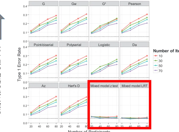
Murayama, Sakaki, Yan, & Smith (2014).
Type I error inflaFon in the tradiFonal by-‐parFcipant analysis to metamomory
accuracy: A generalized mixed-‐effects model perspecFve. JEL:LMC. doi:
10.1037/a0036914 よりFigure 1
to a general conservatism (see supplemental materials on adjusted power analysis).
Simulation 2: A Single-Group Case With Varied
JOL thresholds
Nelson (1984) argued that Goodman and Kruskal’s gamma correlation (G) is preferable because it is insensitive to the place-ments of the thresholds of metacognitive judgplace-ments. In Simulation 1, however, we placed fixed-interval thresholds for metacognitive judgments across participants (i.e., we set five equal-interval threshold values on the JOL dimension such that the continuous JOL are mapped onto a 6-point discrete scale), and these fixed thresholds may have underestimated the usefulness of G. Simula-tion 2 addressed this issue by adopting varied thresholds for JOL ratings across participants.
Method. The simulation was identical to Simulation 1 with a
random item effect, except for one setting. Specifically, rather than use fixed threshold values to determine categorical JOL ratings, we randomly sampled (from a uniform distribution between !1.5 and 1.5) five threshold values for each participant, and used these thresholds to map a continuous JOL values onto categorical JOL ratings on a 1– 6 scale.
Results. The varied thresholds simulation revealed that G and
other metamemory measures still exhibited Type I error rate in-flation (see Figure 3). On the other hand, mixed-effects model analysis kept Type I error rates close to .05, despite the fact that the mixed-effects model assumes an interval scale of measurement. These findings indicate the robustness of mixed-effects modeling to threshold variation in metamemory judgment.
Simulation 3: A Single-Group Case With Dichotomous
JOL Ratings
In some metamemory paradigms, such as feeling of knowing, metamemory judgments are made on a dichotomous scale (e.g., Hart, 1965). Accordingly, literature on measurement of metamemory accuracy has often focused on dichotomous metamemory judgments (Nelson, 1984; Rotello et al., 2008). As such, it is important to examine the performance of the by-participant analysis with a dichotomous independent variable. Because dichotomous judgments carry less information with regard to participants’ true state (MacCallum, Zhang, Preacher, & Rucker, 2002), a mixed-effects model analysis may not exhibit better performance than other metamemory measures specifically adapted for dichotomous variables. In Simulation 3,
G Gw G* Pearson
Point-biserial Polyserial Logistic Da
Az Hart's D Mixed model z test Mixed model LRT
0.0 0.1 0.2 0.3 0.4 0.0 0.1 0.2 0.3 0.4 0.0 0.1 0.2 0.3 0.4 20 40 60 80 20 40 60 80 20 40 60 80 20 40 60 80 Number of Participants Type 1 Er ror R at e Number of Items 10 30 50 70
Figure 1. Type I error rates as a function of number of participants and number of items in Simulation 1, when
random item effect is present. Gw" corrected gamma correlation proposed by Wilson (1974); Logistic " logistic
regression coefficient; Da" a signal detection measure with unequal variance computed by Equation 4; Az"
a signal detection measure with unequal variance computed by Equation 5; D " Hart’s difference score; mixed model z test " z value more than 1.96 with mixed-effects model; mixed model LRT " log-likelihood ratio test with mixed-effects model. The predetermined alpha value (# " .05) is highlighted by the dotted line. See the online article for the color version of this figure.
This document is copyrighted by the American Psychological Association or one of its allied publishers. This article is intended solely for the personal use of the individual user and is not to be disseminated broadly.
7
GAMMA AND MIXED MODELING