A Study on Top-down Search
Algorithms for m -Closest Keywords
Queries Problem over Spatial Web
Yuan Qiu
THE UNIVERSITY OF ELECTRO-COMMUNICATIONS
March 2017
A Study on Top-down Search
Algorithms for m -Closest Keywords
Queries Problem over Spatial Web
Yuan Qiu
Submitted to the Graduate School of Information Systems in partial
fulfillment of the requirements for the degree of
Doctor of Engineering
THE UNIVERSITY OF ELECTRO-COMMUNICATIONS
March 2017
A Study on Top-down Search
Algorithms for m -Closest Keywords
Queries Problem over Spatial Web
APPROVED BY SUPERVISORY COMMITTEE:
CHAIRPERSON:PROF.Tadashi OHMORI
MEMBER:PROF.Yasuhiro MINAMI
MEMBER:PROF.Hiroyoshi MORITA
MEMBER:AP.Hisashi KOGA
MEMBER:AP.Yasuyuki TAHARA
MEMBER:AP.Takahiko SHINTANI
Copyright
By
Yuan Qiu
Abstract
This thesis addresses the problem of m-closest keywords queries (mCK queries) over spatial web objects that contain descriptive texts and spatial information. The mCK query is a problem to find the optimal set of records in the sense that they are the spatially-closest records that satisfy m user-given keywords in their texts. The mCK query can be widely used in various applications to find the place of user’s interest.
Generally, top-down search techniques using tree-style data structures are appropriate for finding optimal results of queries over spatial datasets. Thus in order to solve the mCK query problem, a previous study of NUS group assumed a specialized R*-tree (called bR*-tree) to store all records and proposed a top-down approach which uses an Apriori-based node-set enumeration in top-down process. However this assumption of prepared bR*-tree is not applicable to practical spatial web datasets, and the pruning ability of Apriori-based enumeration is highly dependent on the data distribution.
In this thesis, we do not expect any prepared data-partitioning, but assume that we create a grid partitioning from necessary data only when an mCK query is given. Under this assumption, we propose a new search strategy termed Diameter Candidate Check (DCC), which can find a smaller node-set at an earlier stage of search so that it can reduce search space more efficiently. According to DCC search strategy, we firstly employ an implementation of DCC strategy in a nested loop search algorithm (called DCC-NL). Next, we improve the DCC-NL in a recursive way (called RDCC). RDCC can afford a more reasonable priority order of node-set enumeration. We also uses a tight lower bound to improve pruning ability in RDCC.
RDCC performs well in a wide variey of data distributions, but it has still deficiency when one data-point has many query keywords and numerous node-sets are generated. Hence in order to avoid the generation of node-sets which is an unstable factor of search efficiency, we propose another different top-down search approach called Pairwise Expansion. Finally, we discuss some optimization techniques to enhance Pairwise Expansion approach. We first discuss the index structure in the Pairwise Expansion approach, and try to use an on-the-fly
kd-tree to reduce building cost in the query process. Also a new lower bound and an upper bound are employed for more powerful pruning in Pairwise Expansion.
We evaluate these approaches by using both real datasets and synthetic datasets for dif-ferent data distributions, including 1.6 million of Flickr photo data. The result shows that DCC strategy can provide more stable search performance than the Apriori-based approach. And the Pairwise Expansion approach enhanced with lower/upper bounds, has more advan-tages over those algorithms having node-set generation, and is applicable for real spatial web data.
Contents
1 Introduction 1
1.1 Background . . . 1
1.2 Description about mCK queries problem . . . . 3
1.3 Objective of the thesis . . . 4
1.4 Organization . . . 5
2 Related Works and Problem Setting 7 2.1 Spatial web data . . . 7
2.2 Spatial keyword queries . . . 9
2.3 Spatial indices . . . 11
2.3.1 R-tree . . . 11
2.3.2 Grid . . . 12
2.3.3 Specialized indices for spatial keyword queries . . . 12
2.4 mCK queries . . . 13
2.4.1 Definition . . . 13
2.4.2 Zhang’s Apriori-based top-down search strategy . . . 15
2.4.3 Guo’s approach . . . 19
2.5 Our motivation based on top-down approach . . . 21
3 DCC-NL 23 3.1 Problem setting . . . 23
3.1.1 Objective of this chapter . . . 23
3.1.2 Zhang’s Apriori-based method on bR*-tree . . . 23 i
ii CONTENTS
3.1.3 Our setting . . . 24
3.2 Diameter Candidate Check (DCC) . . . 26
3.2.1 Basic idea of DCC . . . 26
3.2.2 Technical terms . . . 28
3.2.3 DCC in a nested loop method . . . 30
3.3 Further pruning rules using MaxMindist . . . 34
3.4 Experimental evaluation . . . 36
3.4.1 Experimental set-up . . . 36
3.4.2 Evaluation of Synthetic Datasets . . . 38
3.4.3 Evaluation of Flickr Datasets . . . 39
3.5 Summary . . . 40
4 Recursive DCC 43 4.1 Optimization of DCC-NL . . . 43
4.1.1 Objective of this chapter . . . 43
4.1.2 Policy to optimize DCC-NL . . . 43
4.2 Review of DCC-NL search approach . . . 44
4.2.1 Description of DCC-NL . . . 44
4.2.2 The problems of DCC-NL . . . 46
4.3 Recursive DCC and tight lower bound . . . 49
4.3.1 Priority Search Order of Recursive DCC . . . 49
4.3.2 Tight lower bound for pruning . . . 51
4.3.3 Object generation in leaf node-set . . . 52
4.4 Evaluation of RDCC . . . 53
4.5 Summary . . . 56
5 Pairwise Expansion 57 5.1 New Top-down Search Strategy . . . 57
5.1.1 Objective of this chapter . . . 57
5.1.2 Basic idea . . . 57
CONTENTS iii
5.3 Pairwise Expansion method . . . 59
5.3.1 Overview . . . 59
5.3.2 Stage1: Top-down Generation of Object-Pair . . . 60
5.3.3 Stage2: Check of Object-Pair . . . 64
5.4 Preliminary evaluation . . . 70 5.4.1 Experimental Set-up . . . 70 5.4.2 Experimental evaluation . . . 71 5.4.3 Further tests . . . 74 5.5 Summary . . . 74 6 EnhancedPE 77 6.1 Remaining issues of the naive PE method . . . 77
6.2 Discussion about data structure . . . 78
6.2.1 Review of on-the-fly quad-tree . . . 78
6.2.2 Balance tree: on-the-fly kd-tree . . . 82
6.3 Convex-hull as new lower/upper bounds in Pairwise Expansion . . . 88
6.3.1 Motivation . . . 88
6.3.2 Preparation . . . 88
6.3.3 New lower bound . . . 90
6.3.4 New upper bound . . . 93
6.4 Evaluation . . . 95
6.4.1 Performance comparison between quad-tree and QSkd-tree . . . 95
6.4.2 Performance comparison between PE and EnhancedPE . . . 97
6.4.3 Memory consumption test . . . 99
6.5 Discussion . . . 101
6.6 Summary . . . 103
Chapter 1
Introduction
1.1
Background
Nowadays massive web data are attached with geographic location information such as Twit-ter [14] and Flickr [15]. This type of web data associated with both textual and geographic attributes is called a spatial web object (or a geo-textual web object). For example, Figure 1.1 shows a photo data from website of Flickr [15], which is an online photo-sharing service. In this figure, we can see some other information beside the photo itself. There is a passage of descriptive text about the photo in the box area. This can be regarded as the textual attributes of this data. And it also contains a photographed location (displayed on the map) in the ellipse area, which can be regarded as the geographic attributes of it. Thus this photo data is a typical spatial web object.
To these spatial web objects, users are not only interested in the contents of them, but also increasingly consider their spatial aspects. Therefore, retrieval of geographic information by using spatial web objects (denoted as objects, in short) has been studied extensively in recent years [1, 3, 18, 19, 20, 25, 22]. The common way of retrieval is called Spatial Keyword
Queries [23]. Spatial keyword queries usually allow users to enter several keywords, and then
return object(s) that best match these keywords from both textual and spatial perspectives. As a simple example of spatial keyword queries, Google M ap provides a service that users can find the spatial web objects by typing in some keywords. Figure 1.2 shows a search instance when we input ’coffee’ as a query keyword, then the objects which cover the
2 CHAPTER 1. INTRODUCTION
given keywords are returned and shown on the map based on their geographic information.
Figure 1.1: An example of Flickr data
1.2. DESCRIPTION ABOUT MCK QUERIES PROBLEM 3
However, in some cases, there may be no single object that can cover all the user-given keywords. In such circumstances, finding a group of objects to collectively match all query keywords had been considered in some researches of spatial keyword queries [1, 3, 7, 36, 38]. In this thesis, we focus on a typical kind of such spatial keyword queries problem, called
m-Closest Keywords(mCK) Queries, which is proposed by Zhang et al [1] in 2009.
As an introductory example, consider a database D of spatial web objects, and suppose that a user gives m keywords as a query Q. Then, an mCK query under Q, is a query to find the ’optimal’ group of objects Oopt from D, in the meaning that:
(i) each keyword in Q is satisfied by textual attributes of some object in Oopt, and
(ii)the objects in Oopt are, among all groups of objects that satisfy the condition (i),
posi-tioned in the spatially-closest manner.
Intuitively, the ’optimal’ group of objects above is regarded as the best and smallest spatial area that satisfy all keywords of Q.
Next section will describe the mCK query in details.
1.2
Description about m CK queries problem
In the description of [1], given m keywords , an mCK query aims at finding a group of the spatially-closest objects that match these m keywords. The group of objects is called an ’object-set’.
Intuitively, the optimal object-set Oopt of an mCK query must satisfy two conditions
about both textuality and spatiality as follow:
Condition 1: All the user-given keywords must be contained in the text collection of Oopt.
Condition 2: Let S be the set of all the object-sets that satisfy the Condition 1. Then the
objects in Oopt must be placed together in the spatially closest positions, among all
cases of S.
Condition 2 must be rewritten formally. That is, in order to formally measure the closeness of objects in an object-set O, Zhang et al proposed a diameter of O, which is defined as the
4 CHAPTER 1. INTRODUCTION
maximum distance between any two objects in O. If the diameter of O is small, then all the objects in O are positioned more closely. Therefore, the Condition 2 is formalized by saying that the diameter of Oopt must be the smallest among those of all object-sets in S.
We need to explain the above description by showing a typical example. As a specific example of mCK query, suppose that there are 15 objects o1 to o15 in a dataset D. Figure
1.3 shows the spatial distributions of these objects on Google map. We can see these objects are located near the Chofu station, and each object is associated with one of three keywords : ”coffee” (6 objects), ”shopping” (5 objects) or ”convenience store” (4 objects). If an user wants to find a place which contains these three keywords, then the user can use an mCK query for D by issuing Q ={coffee, shopping, convenience store} as query keywords. There are 6× 5 × 4 = 120 combinational sets that can satisfy Q. And we can see the object-set{o4, o7, o8} has the smallest diameter among all the 120 object-sets. Thus {o4, o7, o8} will
be returned to the user. The diameter of the object-set {o4, o7, o8} is the distance between
o4 and o8.
Typically, mCK queries can be used in various location-based services like recommenda-tion of tourist attracrecommenda-tions or real estate to match user’s interests. For instance, mCK query can be applied to the photo data of Flickr. By means of mCK queries we can find a set of photos about all keywords we are interested in, and the locations of these photos will be gathered in a point or an small area, which can be used as recommended information for tourist or others.
1.3
Objective of the thesis
To find the optimal solution of an mCK query, we need to compare all the object-sets. And each object-set is a combination of some objects from a spatial web dataset. Thus suppose there are N objects in the dataset. Then, the number of object-sets is up to O(Nm). Hence
the cost of comparison is expensive. Generally, a top-down search technique using tree-style data structures is appropriate for finding optimal results of queries over spatial datasets, and has been used in various spatial query problems such as nearest neighbor search [24] and multiway spatial join [25, 26], etc. Thus, for the mCK query problem, the study of Zhang et
1.4. ORGANIZATION 5
Figure 1.3: An example of mCK query
al [1] assumed a specialized R*-tree (called bR*-tree) to store all records and proposed a top-down approach which uses an Apriori-based enumeration of node sets in top-top-down process. However there are still some questions to be figured out, we think.
Therefore, our main objective of this thesis is to improve the previous work of top-down search approach for mCK queries with respect to the design of data index and search strategy. We analyze the factors which restrict the search efficiency by clarifying our unique questions to existing methods, and propose four new, more efficient, top-down search methods to solve this problem.
1.4
Organization
6 CHAPTER 1. INTRODUCTION
Chapter 2 reviews related works of mCK queries problem. This chapter first introduces spatial keyword queries over geo-textual web. Then details of mCK queries problem are described, including problem setting and preceding techniques. After that we describe our motivation of this thesis.
Chapter 3 proposes a new search strategy called Diameter Candidate Check(DCC) and an on-the-fly data structure for those questions in Chapter 2. This chapter first outlines basic ideas of DCC strategy. Then a nested loop method using DCC strategy, which is called DCC-NL, is proposed.
Chapter 4 enhances the DCC strategy in a recursive way, which is called RDCC. Moreover, this chapter also introduces an optimized technique incorporated with RDCC method , which uses a new tighter lower bound to improve pruning ability,.
Chapter 5 proposes a new top-down search way Pairwise Expansion(PE). This chapter first discusses limitations of the exploration policy in the preceding chapters, which needs to generate node-sets in top-down process. Then detailed description of PE without node-set generation is given.
Chapter 6 improves PE by using a convex-hull based lower/upper bounds. And a different data structure on-the-fly kd-tree will be discussed in this chapter.
Chapter 2
Related Works and Problem Setting
2.1
Spatial web data
Spatial web data associated with both geographic location and text information can be found everywhere in our daily life. For example, a lot of online social media (or social networking services) such as Twitter and Facebook enable users to post messages with their publishing locations. Figure 2.1 shows a ’tweet’ data from website of Twitter [14]. In this ’tweet’ data, there is a short message with some characters as text information. In addition to this, it also contains a location information where the message is published. Besides, a ’post’ data of Facebook, which is shown in Figure 2.2, also allow users to attach a geotag to the photos as well as some textual tags. In addition, the spatial data for business or PoIs (points of interests) with a name or textual description such as hotels or restaurants also increasingly appeared in web. According to official home page of Google Place API [29], Google declared that it has more than 100 million specific places with detailed information in Google’s ’Places API Web Service’ [29]. Therefore the spatial web data becomes a very important part in the web.
As a formal description, according to [9], a spatial web data is described as o :hψ, λi, where o.ψ is the text property of o in the form of a text message or tags, and o.λ is the location of o by using geographic coordinates. o is denoted by an object from here on.
At the same time, due to these increased sources of spatial data, various web applications that satisfy both contents and spatial requirements are provided to support different services.
8 CHAPTER 2. RELATED WORKS AND PROBLEM SETTING
For example, we can search for a hotel from online hotel reservation services such as ”Jalan” by using a map view (in Figure 2.3). It is more convenient for us to understand the details of the hotels including their locations and other services information. On the other hand, there is a large demand for spatial data on the Web. We can refer to the report in the article of [30] which says ”50 percent of mobile users are most likely to visit shops after conducting a local search, while this number of consumers on tablets or computers is 34 percent.” Thus queries with a spatial intent take up a large proportion in search engines.
Consequently, retrieval about these spatial web data brings us new issues and challenges.
Figure 2.1: An example of tweet
2.2. SPATIAL KEYWORD QUERIES 9
Figure 2.3: Spatial search on Jalan
2.2
Spatial keyword queries
A spatial keyword query is a general concept that allows users to issue some keywords of interest to find the spatial object(s) which can best match their needs about textuality and spatiality.
There ara many specific spatial keyword queries for different needs of users [31, 40, 6, 41, 42, 43]. Some tutorials categorized these queries according to their targets of retrieval [2, 23, 5]. Here we introduce some typical queries to review these spatial keyword query problems based on the tutorial of [5].
Early researches of spatial keyword queries target one individual object or a list of ranked objects in a spatial web dataset [31, 32, 33, 34, 35]. They are generalized as standard queries in [5]. As an typical standard queries, Cong et al proposed a Top-k kNN query(TkQ) [32]. In the TkQ problem, given a query q with a location and a set of keywords, each object o in dataset can be evaluated by two arguments: location proximity and text relevancy [32]. The location proximity of o is determined by the Euclidian distance between o and location of q, and text relevancy of o is computed using the language model of q’s keywords. Then Cong et al used a linear score function of location proximity and text relevancy to give a score to each object. Finally k objects with the highest scores are returned.
10 CHAPTER 2. RELATED WORKS AND PROBLEM SETTING
The standard queries are applicable to the cases of finding several objects, each of which can independently meet user’s needs. A good example is to find some PoIs in location services by using accessible keywords, such as ”comfortable hotel” or ”sushi restaurant”, which are easy to concentrate on one object.
However, in some other cases, the standard queries may not be appropriate. Considering the case that an user may issue the keywords ”station, school, supermarket” to look for a real estate, these keywords are difficult to be covered by an exact place. With a view to these cases, finding a group of objects to match query keywords had been proposed in the researches of spatial keyword queries [1, 10, 9, 3, 7, 4, 36, 37, 38, 39].
One of these researches is the subject of this thesis, m-Closest Keywords(mCK) queries. An mCK query retrieves a set of objects Oopt which covers all the query keywords and each of
them should be close to each other [1]. This query uses a diameter of an object-set O, which is the maximum Euclidean distance between any two objects in O to measure the closeness of O, and minimize the diameter.
Another typical query is so-called collective spatial keyword query that proposed by Cao et al [3]. Similar as the mCK query, a collective spatial keyword query also retrieves the optimal object-set Oopt that must cover all the user-given query keywords. However this
query does not only consider the inner closeness of Oopt, but still need to take into account the
closeness between Oopt and query location. Thus for each object-set O, Cao et al proposed a
linear function of these two closenesses to calculate the ’cost’ of O, and minimized this cost. Actually the collective spatial keyword query is an extension of the mCK query, whose result is the optimal group of objects with a small diameter, and near to the query location.
After that, some other queries to find optimal group(s) of objects such as T op-k Groups
Queries [37] are proposed [4, 36, 38, 39]. Most of these queries measure closeness of object-set
in the same manner as the mCK query. Thus mCK query problem is important and worthy of study.
Consequently, if the standard spatial keyword query is regarded as to find some positions of interests (PoIs), then the retrieval of object group can be considered as finding a region of interests, which may contain various individual PoIs. This can provide users with more abundant quality results in practical applications.
2.3. SPATIAL INDICES 11
2.3
Spatial indices
A spatial index is a kind of organization of spatial data according to their locations. As auxiliary spatial data structures, spatial indices are used to improve the speed and efficiency of spatial queries associating with some specific query algorithms. There have been many studies about spatial indices and a number of different types of spatial indices have been proposed. Here we briefly describe two common types of them: R-tree and grid.
2.3.1
R-tree
An R-tree [48] is a height-balanced hierarchical data structure, which is an extension of B-tree in the multi-dimensional spaces. It divides spatial objects by using minimum bounding
rectangles (MBRs). An MBR R is a ’region’, that means all the spatial objects belong to R
are included in the ’region’ of R, and the ’region’ is minimized. Each of MBR corresponds to an node in R-tree. There are two kinds of nodes: internal nodes and leaf nodes. An internal node of R-tree has some children nodes such that the MBRs of these children nodes must be included in the MBR of it. A leaf node contains pointers to the spatial objects in its MBR.
Figure 2.4 shows an example of R-tree. R4 to R10 are leaf nodes. Each of them corre-sponds with an MBR in the planar space, which tightly bounds some objects in it. R1 to R3 are internal nodes, each of which contains some leaf nodes. R0 is the root node of this R-tree. It is a specific internal node such that the MBR of R0 includes all the objects.
12 CHAPTER 2. RELATED WORKS AND PROBLEM SETTING
There are many variants of R-trees to improve the efficiency of R-tree such as R*-tree and R+-tree, etc. R*-trees optimized the node-splitting method in order to reduce the overlap of MBRs and number of children nodes. Thus it is one of the most widely used in various spatial queries.
2.3.2
Grid
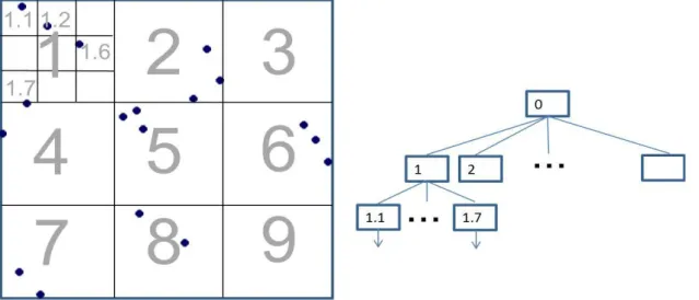
A grid index is a simple structure that divides spatial objects into some equal-sized square or rectangular regions. Each region is called a cell. In some cases, spatial objects are not evenly distributed, thus the cells with dense objects are often subdivided into sub cells until the numbers of all the cells are less than a threshold (or capacity). This type of unbalanced and multi-level grid index is called a hierarchical grid partitioning. Figure 2.5 shows an example of hierarchical grid partitioning. In this figure, all the objects are assigned to 3× 3 = 9 cells. If the capacity is set to 4, then the cell 1 needs to be subdivided into 9 cells again.
Figure 2.5: An example of grid
2.3.3
Specialized indices for spatial keyword queries
For a spatial web object, it has not only spatial but also the textual attributes. Thus, in order to efficiently search these spatial web objects, a lot of new index technologies have been proposed [46, 47, 1]. These indices often use inverted file or bitmap to index the textual
2.4. MCK QUERIES 13
attributes of objects, then combined them with R-tree or grid by using some combination schemas for their geographic attributes. For example, Zhang et al proposed bR*-tree as index structure for mCK queries. The bR*-tree uses R*-tree as a spatial index. And in each node of R*-tree, a keyword bitmap is added to summarize the keywords in the node. Another example of IR-tree, which is widely used in spatial keyword queries, combines R-tree and inverted file in a seamless manner. It can simultaneously handle both the textual and spatial aspects of the spatial web objects, thus the efficiency of query can be improved.
2.4
m CK queries
2.4.1
Definition
According to the original definition of [1, 9], the mCK query (m-closest keywords query) is defined as follows:
[m CK query]: Given a spatial database of objects D ={o1, o2, ..., on} and a query with
m given keywords Q = k1, k2, ..., km, let O ={oi1, oi2, ..., oil}(⊆ D) be a set of objects, termed
an object-set. If an object-set O covers all the keywords of Q, ( ∪
o∈O
o.ψ ⊇ Q), then we say
that O ’satisfies’ Q.
Let also diam(O) = max
ox,oy∈O
dist(ox, oy) (x6= y) , where dist(ox, oy) is the distance between
ox and oy, be termed a diameter of O. Then, the m CK query is defined as a query to find
the object-set Oopt = {oi1, oi2, ..., oil} (l ≤ m) where Oopt has the smallest diameter among
all object-sets O that satisfy Q.
The mCK query aims to find the object-set Oopt such that Oopt satisfies query keywords Q
and the objects in Ooptshould be closest to each other. In this definition, the diameter is used
to measure the closeness of an object-set. As an example, for the object-set O ={o1, o2, o3, o4}
in Figure 2.6, distance between o1 and o4 is the diameter of O.
Actually an object-set O can be regarded as a set of discrete points in the multi-dimensional spaces, and we can use a convex hull of these points in O to represent the amount of space occupied by O. It is intuitive that if the convex hull of O is small, then the objects in O are
14 CHAPTER 2. RELATED WORKS AND PROBLEM SETTING
Figure 2.6: Diameter of object-set
Figure 2.7: Diameter comparison
close to each other. Thus the diameter of convex hull (i.e., the diameter of object-set) is a simple way that can be good at estimating the size of its occupied space. Compared with the other measurement metrics such as area (or volume) size, using diameter can greatly simplify the calculation procedure, especially in high-dimensional space. Therefore the diameter of an object-set is well suited option to represent the its closeness, and this way is used in many other spatial keyword queries which aim for a group of objects [3, 7, 4, 36, 37]. In Figure 2.7 , because the diameter of object-set O1 is less than object-set O2, we can see the objects in
O1 is closer to each other than O2.
2.4. MCK QUERIES 15
2.4.2
Zhang’s Apriori-based top-down search strategy
Generic strategy
Essentially the mCK query can be classified as the problem that find the optimal solution from possible solution space over spatial dataset. For this type of problems, a branch-and-bound technique in a top-down process based on hierarchical data structure has been successful in numerous spatial queries such as nearest neighbor query (NN query) [24], range query [27] and spatial join [25, 26].
We briefly describe a typical branch-and-bound technique of top-down strategy as follow:
Step 1 (Initialization): Use a global variable χ∗ to represent the current optimal solution of the spatial query and initialize χ∗ with +∞ or −∞.
Step 2 (Start): Start from the root node of the hierarchical data structure. Because the optimal solution must exist in the region of root node, choose this region as current solution space SC.
Step 3 (Check and Pruning): For current solution space SC, if it exists no better
solu-tion than χ∗ in SC, then prune the branch of SC. Otherwise, goto Step 4.
Step 4 (Branching): If SC is an internal-node, then divide SC into some partial regions
as candidate solution spaces by using its children nodes. Otherwise if SC is a leaf-node,
then enumerate all the solution χ in SC and compare with χ∗ for each χ: if χ is better
than χ∗, then update χ∗ with χ.
Step 5 (Selection of Candidate): Choose one from the candidate solution spaces as cur-rent solution space SC, then return to Step 3.
Step 6 (Termination Test): Stop if there is no candidate solution spaces. Finally χ∗ is the optimal solution.
Zhang’s approach
According to the above description, Zhang et al proposed a top-down exploration approach taking advantage of a special R*-tree called bR*-tree [1](2009). The bR*-tree is an extension
16 CHAPTER 2. RELATED WORKS AND PROBLEM SETTING
of the index structure of R*-tree . Beside the node MBR of R*-tree, each node N in bR*-tree is augmented with two additional information: keyword bitmap and keyword M BR.
• keyword bitmap: keyword bitmap is a bitmap that summarize the keywords in the
node N . Each bit bi shows that whether a keyword ki exists in N . If bi = 1, then
there exists at least one object associated with keyword ki in N . Otherwise, there is
no object of ki in N .
• keyword MBR: For each keyword ki, the keyword M BR of ki is the minimum bound
rectangle of all the objects in N that are associated with ki.
(a) Data distribution and bR*-tree (b) Search space tree
(c) Keyword bitmap and keyword MBR
Figure 2.8: An example of Apriori-Z
Figure 2.8(a) is an example of the bR*-tree for the objects associated with four keywords
A,B,C and D. In this bR*-tree, root node R0 has five children nodes R1 to R5. Each node
2.4. MCK QUERIES 17
bitmap and keyword M BR are also attached in each node(Figure 2.8(c)). For example of
Figure 2.8(c), in node R2 the keyword bitmap = 1100 denotes that R2 contains objects only
associated with keyword A and B, not C and D. Accordingly, the keyword M BR of A and
B are the spatial bound of all the objects with keyword A and B, respectively.
Zhang et al used the bR*-tree to index all the objects and proposed a top-down search approach based on this bR*-tree. Next we describe this top-down approach.
Different from the typical spatial queries such as NN queries or range queries, the result of mCK query is a set of objects, thus the solution spaces are not confined in one node of bR*-tree. For this reason, Zhang et al used a set of nodes, termed as a node-set, as a solution space in the search process. That means for a solution (an object-set O) in a solution space (a node-set N ), each object of O must belong to one node of N and each node of N must contain at least one object of O.
Therefore in the branching procedure of top-down process for the mCK query problem, the solution space SC is divided into all the possible sub solution spaces (sub node-sets), each
of which is a combination of children nodes of SC. For example, Figure 2.8(b) is the search
space tree of the bR*-tree in Figure 2.8(a). In Figure 2.8(b), we can see each branch of the root node R0 is a subset of{R1, R2, ..., R5} such as {R1, R2, R4}. Here the size of the node-set
is m at most, because an object-set is compose of at most m objects. In addition, these sub node-sets are generated as an Apriori-style way which has been used for mining frequent itemsets. Thus the enumeration of these sub node-sets follows the order from length-1 (one MBR) to length-m (m MBRs). Due to this, we call Zhang’s top-down approach as Apriori-Z approach.
Apriori-Z
In Apriori-Z, a global variable δ∗ is denoted as the current smallest diameter among the object-sets explored so far. Then in the pruning procedure of top-down process, Zhang et al proposed three pruning rules for a node-set N as follow to decide whether it can be pruned.
Pruning rule 1: If N does not contain all the query keywords, then there exists no object-set that contains all the keywords in N . Thus N can be pruned directly.
18 CHAPTER 2. RELATED WORKS AND PROBLEM SETTING
Pruning rule 2: If there exists two nodes ni, nj ∈ N such that the minimum distance
between ni and nj is greater than δ∗, then N can be pruned. That is because the
minimum distance between ni and nj is an lower bound of distances between any two
objects oi and oj (oi ∈ ni, oj ∈ nj). Hence it is also the lower bound of the diameters
of possible object-sets. If this lower bound is greater than δ∗, there exists no object-set with diameter than δ∗ in N .
Pruning rule 3: If the distance between two keywords are greater than δ∗, which means for any object oi associated with keyword kiand oj associated with keyword kj in N , we
can always find that dist(oi, oj) is greater than δ∗, then N can be pruned. The keyword
MBRs in each node of N are used to calculate the distances between two keywords.
In the selecting procedure of top-down process, Zhang et al traversed the search space tree in the depth-first order. That means if a node-set N as the current solution space cannot be pruned, then immediately access N ’s sub node-sets.
In consequence, we summarize Apriori-Z approach as follow:
Step 1 (Initialization): Use a global variable δ∗ to represent the current smallest diame-ter. δ∗ is initialized as follow: first find the smallest node NI that contains all the query
keywords among all the nodes of bR*-tree. If NI is an internal-node, then initialize
δ∗ with the diagonal distance of NI; if NI is a leaf-node, then initialize δ∗ with the
smallest diameter in NI by exhaustively generating all the object-sets.
Step 2 (Start): Start from the root node-set {root} of the bR*-tree. choose it as current node-set NC.
Step 3 (Check and Pruning): For current node-set NC, if it can be pruned by the three
pruning rules, then skip NC and repeat to check next candidate node-set. Otherwise,
goto Step 4.
Step 4 (Branching): If all the nodes in NC are leaf-nodes, then enumerate all the
object-sets in NC and compare each diameter δ with δ∗ : if δ < δ∗ , then update δ∗ with δ.
2.4. MCK QUERIES 19
Step 5 (Selection of Candidate): Choose the first sub node-set in a depth-first way, then return to Step 3.
Step 6 (Termination Test): Stop if all the candidate node-sets are checked. Finally δ∗ is the optimal diameter.
2.4.3
Guo’s approach
In the study of [9] in SIGMOD 2015, Guo first theoretically proved that the problem of
mCK queries is NP-hard. Then they mainly focused on several algorithms for finding the
approximation solution of mCK queries problem. At the end of their study , they also presented an exact algorithm by utilizing the result of the approximation algorithm. Here we summarize their algorithms, according to the description of their paper [9].
The first proposed algorithm is called Greedy Keyword Group(GKG). Given a query
Q = {k1, k2, ..., km}, make a set of object collections C = {C1, C2, ..., Cm} such that each Ci
(i∈ {1, ...m}) is the collection of objects associated with keyword ki. Then GKG first chooses
the collection having the smallest size inC, denoted by Cinf. Next, for each object o in Cinf,
GKG finds the nearest object from o, from within Cj for each keyword kj (kj ∈ Q − o.ψ).
Then these nearest objects with o form one object-set covering all the keywords of Q. Thus, after all of these object-sets from Cinf are generated, GKG chooses the object-set GGKG
which has the smallest diameter as the answer. Guo proved that this answer is not larger than twice of the diameter of the optimal result.
Next, Guo proposed a series of algorithms which can get better approximation ratios than GKG. The basic idea of these algorithms is to construct a M inimum Covering Circle (M CC) for an object-set G , denoted by M CCG. M CCG is defined as the circle that encloses
all the objects of G with the smallest diameter. Then the diameter of M CCG is used as an
approximation of G’s diameter.
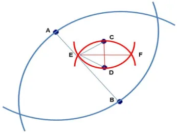
In [9], Guo denoted the diameter of the circle M CCG by φ(M CCG), and denoted the
diameter of object-set G by δ(G). The relationship between φ(M CCG) and δ(G) can be
deduced by using a theorem (in [49]) that M CCGcan be determined by at most three object
20 CHAPTER 2. RELATED WORKS AND PROBLEM SETTING
(a) M CCG1 is determined by two points (b) M CCG2 is determined by three points
Figure 2.9: Example of two diameters (This figure is derived from Fig.2 of [9])
M CCG is determined by only two object points, then the line segment connecting those two
points must be a diameter of the circle (see Figure 2.9 (a)). If M CCGis determined by three
object points, then the triangle consisting of those three points is not obtuse (see Figure 2.9 (b)). Based on these observations, Guo derived out the following inequality relation [9].
√
3
2 φ(M CCG)≤ δ(G) ≤ φ(MCCG). (2.1) Accordingly, the search policy of Guo’s approximate algorithms is to find the M CC having the smallest diameter such that the object-set in the M CC must cover all the query keywords of Q.
The above M CC is called Smallest Keywords Enclosing Circle, denoted by SKECQ.
And the object-set in SKECQ is denoted by GSKEC. Then according to the inequation (2.1),
Guo proved that δ(GSKEC) ≤ φ(MCCSKEC) ≤ √23δ(Gopt) where δ(Gopt) is the diameter of
the optimal result. Thus the approximation ratio can be reduced to √2
3 by using SKECQ as
approximate solutions.
2.5. OUR MOTIVATION BASED ON TOP-DOWN APPROACH 21
which are called SKEC, SKECa and SKECa+, respectively. Basically, according to the above explanations, the circle of SKECQ is determined by two or three object points. In
algorithm SKEC, Guo considers the set of objects that contain at least one query keyword, denoted by O0, and then for each object o∈ O0 as a seed point, o is combined with other one or two points to determine a circle and check if this circle contains all the query keywords. In SKEC, some objects which are combined with o can be pruned out by using the result of algorithm GKG.
Next, Guo uses algorithm SKECa and SKECa+ to find SKECQapproximately. SKECa
uses a binary search to find the approximate smallest keywords enclosing circle for each o∈ O0.
SKECa first sets a circle with an upper bound D of a diameter and sets o as an object
lo-cated on the boundary of the circle. Then this circle is rotated around o clockwise and tests whether or not it can cover all the query keywords at a particular position. If it can, then
SKECa tries to test a smaller D; otherwise, it enlarges D. This process is repeated until
the error tolerance ratio of binary search is converged within a small value. After all the ob-jects o are checked, the approximate answer of SKECQ can be found. The other algorithm
SKECa+ enhanced SKECa. In SKECa+, the binary search process is performed on all
objects in O0 together,instead of the testing on each of them separately. Thus the checking cost can be reduced.
At last, Guo also proposed an exact algorithm. This algorithm sets a circle with diameter
2
√
3φ(GSKECa) where GSKECais the answer of algorithm SKECa+. Then the circle is rotated
around each o clockwise, and once it covers all the query keywords, then the algorithm exhaustively enumerates all the object-sets in the circle. Finally, the exact result can be found.
2.5
Our motivation based on top-down approach
In this chapter, we introduced mCK query problem and some previous researches for it. As a spatial query problem, the top-down search by using a spatial index is a kind of fundamental method. Though Guo’s approach which is different from top-down style is good at finding the approximation solution of mCK query problem, when considering further requirements
22 CHAPTER 2. RELATED WORKS AND PROBLEM SETTING
of various spatial searches such as finding top-k closest object-sets, top-down search is surely an useful technique for these extensions.
However the existing Apriori-Z approach is a straightforward top-down method, which combines the node-sets of bR*-tree in an apriori way level-by-level with some pruning rules. There are some apparent questions in this approach.
• Apriori-Z decides whether or not a given node-set can be pruned out through the
comparison of the N ’s lower bound and the current smallest diameter δ∗ in pruning rule 2 and 3. Hence the δ∗ is an important factor that influences the pruning efficiency. If an smaller δ∗ can be found in an early stage, then more node-sets can be pruned out. Otherwise, it needs to generate enormous amount of object-sets and node-sets such that the search efficiency is poor. However, the Apriori-based enumeration of sub node-sets cannot guarantee that the smaller object-set will be enumerated firstly especially in the skewed distribution.
• Apriori-Z uses a bR*-tree to store all the objects. However the bR*-tree is not applicable
to the real spatial web which are frequently updated like Flickr and Twitter data. Moreover for the practical cases of mCK query, such as that we may want the results from different datasets (like Twitter and Flickr) simultaneously, we need a more flexible index to satisfy various user’s requirements.
Therefore, there remain much rooms for us to consider deeply and explore more sophisti-cated top-down approaches for mCK query problem. We explore these sophistication in the following chapters.
Chapter 3
DCC: A New Top-down Search
Strategy with a Priority Order
3.1
Problem setting
3.1.1
Objective of this chapter
In chapter 2, we discussed some problems in the Apriori-Z approach for mCK query problem. Thus the objective in this chapter is to ameliorate these problems in two aspects:
1) Consider a new technique to organize these spatial web data for more practical situation. 2) Improve the pruning ability of search space by enumerating the node-sets in a priority order.
3.1.2
Zhang’s Apriori-based method on bR*-tree
In the study of [1], Zhang et al used a specialized R*-tree, a bR*-tree, to store all records in preparation, and proposed an Apriori-based enumeration of MBR combinations. However, this assumption of R*-tree is not applicable to all cases; Twitter or Flickr just provides only ’bare’ records having location information, or, at most, some major services like Google Maps only provide grid-style partitioning. In addition the Apriori-based enumeration method performs well especially when one MBR (or, one object) satisfies multiple keywords. In contrast, the method is weak when any set of mutually-close MBRs does not satisfy Q. In
24 CHAPTER 3. DCC-NL
that case, the Apriori must enumerate too many itemsets of MBRs. To avoid it, the method depends on how well a bR*-tree clusters the optimal answer into one MBR of an upper level.
3.1.3
Our setting
In this chapter, we do not expect any prepared data-partitioning, but assume that we create a grid partitioning from necessary data only when an mCK query is given. Under this assumption, we propose a new search-strategy termed Diameter Candidate Check (DCC), and show that DCC can efficiently find a better set of grid-cells at an earlier stage of search, thereby reducing search space greatly.
Figure 3.1 is our assumption of executing mCK queries over spatial web objects. When a query of m-keywords is submitted, we load objects associated with each keyword ki from
one or multiple datasets and then create a hierarchical grid partitioning Gi for each ki. Thus
m grid indexes are built.
Figure 3.1: On-demand creation of grid partitioning
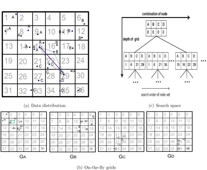
Figure 3.2(a) is an example of spatial distribution of some objects, and each object is associated with one keyword among A, B, C, D. When Q = {A, B, C, D} is given, four hierarchical grids GA, GB, GC, GD are created as shown in Figure 3.2(b). In a hierarchical
grid partitioning of a fixed degree(4x4=16, as an example) of equi-sized partitioning at each level, each cell of the grid partitioning is uniquely denoted by an ordinal integer i. (e.g., let
3.1. PROBLEM SETTING 25
i = 0 be the root node. Then i = 17 is the 1st cell of the level of 2(=1 + 17 mod 16)). In the
following, the symbol A[i] refers to the i-th cell of the grid corresponding to the keyword A. Such A[i] is termed a node. When Q is {A, B, C, D}, the set of nodes {A[i], B[j], C[k], D[l]} is termed a node-set.
Furthermore, in the following, in each grid Gi for a keyword ki, each cell is given an
additional MBR that contains all objects stored in the grid-cell. This is equal to the
keyword-MBR of bR*-tree. We use these keyword-keyword-MBRs for estimating distance between cells.
Next, Figure 3.2(c) is the search space for finding the optimal node-set under A, B, C, D using a naive nested loop search algorithm. Here we use δ∗ to denote the current minimum diameter and it is initialized to ∞. Then this algorithm is written as follow:
Algorithm 1: Nested-Loop(curSet)
curSet is an m-sized node-set each of node in curSet belong to a grids Gi .
Step 1: If the curSet is an internal node set and the distance between every two nodes
∈ curSet is less than δ∗, we first put all child-node(s) (i.e. child grid-cells) of each
internal node into a list, respectively; and then start to enumerate new child node-sets according to the nested loop of these child-node lists in the order of the ordinal integers of cells. Every time when a new child node-set is generated, we recursively invoke this Nested-Loop algorithm using the new node-set as curSet. When all breaches are tested, return δ∗.
Step 2: If the curSet is an m leaf node-set and the distance between every two nodes
∈ curSet is less than δ∗, we exhaustively enumerate all the object-sets and find the
minimum diameter of object-set, then update the value of δ∗ to this diameter.
In the example of Figure 3.2(c), we start from the root node-set {A[0], B[0], C[0], D[0]}. Then the node-set{A[1], B[1], C[2], D[2]} becomes the first child node-set generated, because
A and B exist firstly in the 1st cells but C and D appear firstly in the 2nd cells. In case of a
naive nested loop search over the given keyword ordering of A, B, C, D on these hierarchical grids, the search recursively proceeds in the depth-first order in the tree of the search space.
26 CHAPTER 3. DCC-NL
(a) data distribution (c) the search space of mCK query
(b) m independent grids structure
Figure 3.2: grid and search space of m-CK
naive approach is too expensive. Furthermore, as a disadvantage of using a grid, the grid structure is often weak in clustering correlated objects in one grid-cell (the over-splitting problem). Thus we must give a higher priority of search to a better set of grid-cells during the recursive search in the search space of Figure 3.2(c).
3.2
Diameter Candidate Check (DCC)
3.2.1
Basic idea of DCC
In the search space of Figure 3.2(c), two factors affect the efficiency of node-set enumeration. One factor is the order of enumerating node-sets. An ideal way is to test a ’better’ node-set with higher priority in the search space; a ’better’ node-set is that having a smaller
3.2. DIAMETER CANDIDATE CHECK (DCC) 27
(a) example of a data set (b) search space and order of node-sets
Figure 3.3: search method of the mCK query
diameter. This leads to finding an object-set having a smaller diameter, which can prune out unnecessary node-sets. We should explore such a desirable node-set as early as possible.
As an example, let us consider a data distribution of Figure 3.3(a) and the corresponding search space of Figure 3.3(b). Actually, there are four independent grids for A, B, C, D in Figure 3.3(a), but we visualize these grids by one virtual grid of Figure 3.3(a).
Figure 3.3(b) shows which node-sets (by combining the cells of the first-level partitioning) are enumerated by the naive nested loop method of Algorithm 1.
In this example, the smallest diameter really exists in the node-set{A[6], B[7], C[10], D[11]} at the first level of grid-partitioning. Clearly, we should choose this ’better’ node-set firstly in Figure 3.3(b), from among all the node-sets of the first-level cells. Namely this ’bet-ter’ node-set should be given a higher priority in the exploration of the search space. This priority-based search is not achieved either by the naive nested loop or the Zhang’s method. In case of using a nested-loop style search in the search space of Figure 3.3(b) or Fig-ure 3.2(c), another expensive factor is the order of keywords to be tested. Let δ∗ be the currently-found minimum diameter in the search process. Suppose we test a node-set
{A[i], B[j], C[k], D[l]} in the nested loop of keyword-ordering of A, B, C, D. Then, if the
minimum distance between C[k] and D[l] is larger than δ∗, the search process will repeat expensive test of other combinations of useless node-sets. Thus a fixed global ordering of
28 CHAPTER 3. DCC-NL
keywords must be avoided in the search process.
To overcome these factors, we propose a search strategy called Diameter Candidate Check (DCC). DCC is aimed to find a node-set having a smaller diameter as quickly as possible and reduces the search space.
The basic idea of DCC is as follows: The goal of mCK query is to find the smallest diameter, and the diameter is determined by two objects ox, oy. Thus, rather than
enumer-ating the m-sized object-sets (or, node-sets) directly, we firstly enumerate all pairs made of two objects, hox, oyi, (or two child-nodes, hnx, nyi,) from an inputted node-set, and sort
the pairs in the ascending order of their possible diameter’s lengths. Each pair is called a
diameter-candidate. Next, in the sorted order of smaller (=better) diameter-candidates, we
pick up a diameter-candidate and generate a new object-set (or, a child-level node-set) from the diameter-candidate, and recursively test the child node-sets, in a top-down manner, if necessary.
By this strategy, due to the ascending sort of diameter-candidates, a node-set having a smaller diameter is tested with a higher priority in the search space. Furthermore, the enumeration of all diameter-candidates is much less expensive than that of all m-sized object-sets.
It is a basic idea to use a pair of ”closer” objects as a key to reduce the search space in various spatial keyword query problems. This idea is also used in the pairwise distance-owner finding in the MaxSum-Exact algorithm of Collective Spatial Keyword Query (CoSKQ,[7]), which is a problem to find the best disc of objects whose center is a given query-point and where the disc must also cover given m-keywords. Their algorithm depends on NN-queries from the query-point or some data-objects by using an IR-tree. In contrast, the mCK problem has no query-point, and our originality of DCC exists in the point that we explore and reduce the search space in a top-down manner without any query-point, by using DCC on dynamically-created hierarchical grid partitions.
3.2.2
Technical terms
To implement DCC, we prepare some technical terms.
3.2. DIAMETER CANDIDATE CHECK (DCC) 29
written as nwi) be a grid-cell associated with a keyword wi. Then, M axdist(nw1, nw2) is the
maximum distance between two rectangles of nw1 and nw2, which are MBRs in the grid-cells
of w1 and w2. M indist(nw1, nw2) is the minimum distance between the same MBRs of nw1
and nw2.
When m-keywords {w1, w2, ..., wm} are given as a query, we define MaxMaxdist and
M axM indist of a node-set N ={nw1, nw2, ..., nwm}, as follows:
Definition 1: For a node-set N ={nw1, nw2, ..., nwm} under m-keywords,
• MaxMaxdist of N is defined as:
M axM axdist(N ) = maxnwi,nwj∈NM axdist(nwi, nwj).
• the pair of nodes hnwi, nwji is said to be the diameter pair of N if dist(nwi, nwj) =
M axM axDist(N ).
• MaxMindist of N is defined by
M axM indist(N ) = maxnwi,nwj∈NM indist(nwi, nwj).
Figure 3.4: MaxMaxdist and MaxMindist
M axM axdist is an upper bound of all possible diameter’s lengths that are derived from
the node-set N . M axM indist(N ) is a lower bound of diameter’s lengths which can be found from N . Figure 3.4 shows their examples of N = {nw1, nw2, nw3}. The pair hnw1, nw3i is the
30 CHAPTER 3. DCC-NL
3.2.3
DCC in a nested loop method
We here describe the implementation of DCC strategy in a nested loop search algorithm. This algorithm is called DCC-NL. DCC-NL uses a nested loop method over all keywords in order to generate and test a new node-set from a diameter-candidate.
DCC-NL has three steps in the process, as shown in Figure 3.5. In the following, we explain the case of four keywords A, B, C, D of Figure 3.2(b) as an example. It is given a node-set NI as the input, and finally returns the minimum diameter. It starts from the root
node-set N0 ={A[0], B[0], C[0], D[0]}, where all nodes are the level-0 grid-cells:
Figure 3.5: workflows of DCC three steps
[step1 : Candidate Enumeration]
We assume that in the inputted node-set NI = {nw1, nw2, ..., nwm}, all nwi’s are non-leaf
nodes. (The other cases are described later.) Then, for each keyword wi, we first find all
child-nodes (i.e., = child grid-cells) which satisfy wi in the node nwi ∈ NI, and put these
child-nodes into a corresponding list Lwi. Next, from every two different lists Lwi and Lwj,
we generate all pairs of child-nodes, by picking one from each list. These pairs are called the
diameter candidates (denoted as DC, in short).
As an example, in Figure 3.6(a), if we use the root node-set as the input, we can get four child-node lists LA, LB, LC, LD corresponding to keyword A, B, C, D. Then four DCs,
3.2. DIAMETER CANDIDATE CHECK (DCC) 31
(a) child-node lists
(b) example of DC and Check
32 CHAPTER 3. DCC-NL
hA[1], B[1]i, hA[1], B[6]i, hA[2], B[1]i, hA[2], B[6]i, are generated from the list LAand LB. Also
six DCs, hB[1], C[2]i, ..., hB[6], C[6]i, are done from LB and LC. Thus we finally generate 37
pairs in total.
Thereafter we sort these DCs by the ascending order of M axdist(DC). Note that if the size of each list Lwi is s, the number of DCs is (mC2 × s
2), which is much less than the
amount of possible node-sets (= sm).
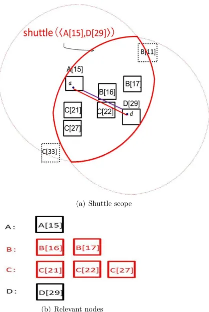
[step2 : Diameter Candidate Check]
We pick up a DC = hni, nji, from the top of the sorted list of DC’s, and check if this
DC cannot become a diameter pair of any child node-set of NI. If so, we will not need to
consider this DC.
There are three points to be checked: they are checked in the order of (2-1) to (2-3). If any one of the points holds, the DC is removed and we return to checking the next DC from the sorted list.
(2-1) If the DC hni, nji is such that Mindist(ni, nj) ≥ δ∗ (δ∗ is the current minimum
diameter), no node-set which is generated from this DC can give an object-set having a diameter < δ∗. Thus we remove this DC and go to the next DC.
(note: This reduces the overhead factor of testing node-sets by the fixed global order of keywords, as described in Section 3.2.1.)
(2-2) Next, we try to generate a node-set ND from the DC hni, nji. (ND is a child
node-set of the inputted node-node-set NI in the search space.) If ND is successfully created, the DC
must be included within ND and be the diameter pair of ND. This requires that every node
n∗ ∈ ND except the two nodes of the DC must satisfy both:
M axdist(n∗, ni) < M axdist(ni, nj) and
M axdist(n∗, nj) < M axdist(ni, nj).
The above condition can be said as follows: every n∗ ∈ ND must be a node included
in the shuttle scope (red) drawn in Figure 3.6(b), where this shuttle scope represents the above condition. This shuttle scope is uniquely determined by a DC, thus being denoted by
Shuttle(DC). In order to compose ND from a given DC, we need not consider any nodes
which are outside the Shuttle(DC).
3.2. DIAMETER CANDIDATE CHECK (DCC) 33
C[3], C[6] in LC and D[2] in LD are outside the Shuttle(hA[1], B[6]i). Thus we ignore these
nodes for generating ND from the DC.
As a result, the step (2-2) is as follows: we check if there exists any keyword wi such that
all the node associated with wi are outside Shuttle(DC). If such wi exists, we remove the
DC and go to the next DC.
(2-3) Next, let the DC be hni, nji and consider the Shuttle(hni, nji). For every two
keywords wx, wy ∈ Q − {wi, wj}, we check the following constraint:
there must exist some two nodes nx, ny where nx ∈ Lwx, ny ∈ Lwy such that both nx, ny are
included in Shuttle(DC) and M axdist(nx, ny)≤ Maxdist(ni, nj). If this constraint fails for
some wx, wy, then the DC hni, nji cannot become a diameter pair any more. Thus, the DC
hni, nji is not necessary to be considered, and the next DC is checked.
As an example, in Figure 3.6(b), both M axdist(C[2], D[5]) and M axdist(C[2], D[6]) are larger than M axdist(A[1], B[6]). Thus the DC hA[1], B[6]i is removed, and we go to the next
DC.
[step3 : Node-Set generation]
After the step 2, we generate a new child node-set ND from the current DC. To do so, we
take a combination of the child-nodes in Shuttle(DC) by using a nested loop method over all Lwi’s of (m− 2) keywords (except the keywords of the DC). During this process, we must
skip over such a node-set that some two nodes in the combination have a larger M axdist than M axdist(DC). Each time when we get an output of the combination over the (m− 2) keywords, the output is merged with the DC, and is used as the ND; i.e., we recursively
invoke DCC-NL(ND).
As the last comment, if all the nodes of the input node-set are leaf-nodes in the step1, each leaf-node is decomposed into individual objects and the above procedure is used. If some node in the input is a leaf and some is not, then the decomposition of the leaf-nodes is skipped over until all nodes in N become leaf-nodes.
According to the above, we summarize the DCC-NL algorithm as Algorithm 2.
34 CHAPTER 3. DCC-NL
curSet is an m-sized node-set each of node in curSet belong to a grids Gi .
Step 1: If the curSet is an internal node set and the distance between every two nodes
∈ curSet is less than δ∗, we enumerate all the node-pairs as DCs and sort them. For
each DC hni, nji in these DCs do:
1.1 Test the step2 for the DC hni, nji.
1.2 If the step2 judges the DC hni, nji must be skipped over, we test the next DC;
otherwise, go to 1.3.
1.3 Generate all (m− 2)-sized node-sets among nodes in Shuttle(hni, nji). Every time
we get an (m− 2)-sized node-set Nm−2 where M axdist between every two nodes
∈ Nm−2 is less than M axdist(ni, nj), we merge Nm−2 and DC hni, nji into an
m-sized node-set and use it as curSet, and we recursively invoke DCC-NL algorithm.
Step 2: If the curSet is an m-sized leaf node-set and the distance between every two nodes
∈ curSet is less than δ∗, we enumerate all the object-pairs as DCs and sort them. For
each DC hoi, oji in these DCs :
2.1 Check the step2 by setting hoi, oji as a DC.
2.2 If DC hoi, oji is judged to be skipped over, we go to the next DC; otherwise, go
to 2.3.
2.3 Generate (m− 2)-sized object-sets. Once we get a (m − 2)-sized object-set Om−2
that the distance between every two objects ∈ Om−2 is less than Dist(oi, oj), we
set δ∗ to Dist(oi, oj), and return.
3.3
Further pruning rules using MaxMindist
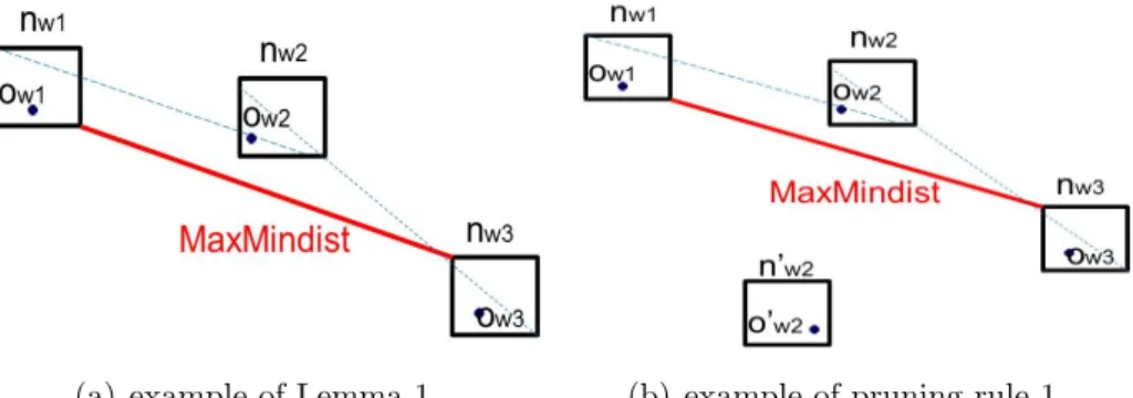
We can consider further pruning rules, which filter out unnecessary node-sets. Firstly, the following lemma holds:
Lemma 1 : Given a node-set N = {nw1, nw2, ..., nwm}, assume that some node nwi ∈ N
3.3. FURTHER PRUNING RULES USING MAXMINDIST 35
not necessary to compute the diameter of N . (Thus nwi can be virtually removed from every
descendent node-set of N .)
In Figure 3.7(a), for the node-set N ={nw1, nw2, nw3}, MaxMindist(N) = Mindist(nw1,
nw3), and both M axdist(nw2, nw1) and M axdist(nw2, nw3) are less than M axM indist(N ).
Therefore, for any object-set {ow1, ow2, ow3} generated from N, dist(ow1, ow3) must be the
largest. Thus all ow2’s in nw2 are not necessary to compute the diameter.
By the lemma 1, we consider two pruning rules:
Pruning Rule 1 Given a node-set N = {nw1, nw2, ..., nwm}, assume that nodes in N
can be classified into two groups {nwa, ..., nwb,|nwc, ..., nwd}, where nwc, ..., nwd are the nodes
which can be removed by lemma 1 and nwa, ..., nwb are not removed. Then we need not test
any other node-set N0 where N0 contains {nwa, ..., nwb}.
In Figure 3.7(b) where N = {nw1, nw2, nw3}, we can remove nw2 from N by Lemma 1.
Then, we can skip over the test of another node set N0 = {nw1, n0w2, nw3}. It is because the
diameter created from N0 is never smaller than that computed from N .
Pruning Rule 2 : If a node-set N is generated from a DC hnwi, nwji and all the nodes
in N except nwi and nwj can be removed by Lemma 1, then any other node set which is
generated from this DC can be pruned out.
Pruning Rule 2 is a special case of Pruning Rule 1. Once a node-set satisfies Pruning Rule 2, we can use only the two nodes of DC for computing the diameter. Furthermore the remaining other node-sets from this DC can be skipped over.
(a) example of Lemma 1 (b) example of pruning rule 1
36 CHAPTER 3. DCC-NL
3.4
Experimental evaluation
3.4.1
Experimental set-up
Here we evaluate our algorithm over synthetic datasets and real datasets.
The synthetic datasets consist of two-dimensional data points where each point has only one keyword. We generated 1000 data points for each keyword in advance, up to 100 key-words. The x- and y- values of a data-point are in [0, R], taken from a square of the side-length
R. As for these synthetic datasets, we prepared a separate data-file for each keyword. When
a query of m-keywords is given, we build m grids from the necessary files, as explained in Figure 3.1. We use three types of data-distribution:
1) uniform distribution: All coordinates of data points are randomly generated (Figure 3.8(a)).
2) normal distribution with σ = 14R: For each keyword, we randomly generate one point
as the reference point, and then all the data points associated with this keyword are generated so that the distance to the reference point follows a normal distribution (Figure 3.8(b)). We set the standard deviation σ = 14R.
3) normal distribution with σ = 1
8R: The same as 2) except that σ = 1
8R (Figure 3.8(c)).
This is the case of much higher skew than that of σ = 14R.
We also employ a real dataset which collects 46,303 photo records from Flickr in Tokyo area. Each photo record contains a geographic information, which is used as the x- and y-values of the data-point. And each record is associated with 1 to 73 tags that can be viewed as keywords of data-point. As an example we choose 4 keywords sakura(red), river(green),
temple(blue), shrine(yellow), and the distribution is shown in Figure 3.8(d). As for the
Flickr data, we stored them in MongoDB, and we prepared keyword indices at first. When a query is given, we load necessary data as shown in Figure 3.1.
As a grid-partitioning of Section 3.1.2, we defined that each cell is divided when the number of data points is greater than 100. The fan-out is set to 100 (= a square of 10 × 10). Note that the grid partitioning is created dynamically when a query is given.
We also implemented the Zhang’s Apriori-based algorithm for the comparison. We execute all algorithms under our grid-partitioning setting of Section 3.1.2. We execute the Zhang’s
3.4. EXPERIMENTAL EVALUATION 37
(a) uniform distribution (b) normal distribution of σ = 1
4R
(c) normal distribution of σ = 18R (d) Flickr photo data distribution
Figure 3.8: data points distribution
method by making one grid structure of Figure 3.2(a). This is fair because our grid still keeps keyword-MBRs in each grid-cell. We implemented all the algorithm in Java with version 1.7 on a machine with an Intel(R) Xeon(R) CPU of 2.6GHz and 12GB of RAM ,running the linux vine 5.2. The performance measure is the average response time (ART). The ART includes all time of data access, grid creation and search execution. For each m, we randomly chose
m keywords 10 times and takes ART.
The algorithms we test are:
• Apriori-Z: Zhang’s Apriori-based algorithm • Nested-Loop: the naive nested loop algorithm


![Figure 2.9: Example of two diameters (This figure is derived from Fig.2 of [9])](https://thumb-ap.123doks.com/thumbv2/123deta/9842928.974273/33.892.181.735.137.472/figure-example-diameters-figure-derived-fig.webp)
![Figure 3.5: workflows of DCC three steps [step1 : Candidate Enumeration]](https://thumb-ap.123doks.com/thumbv2/123deta/9842928.974273/43.892.290.630.421.744/figure-workflows-dcc-steps-step-candidate-enumeration.webp)