Development of Quasi-static Curve Negotiation Analysis Procedure Considering Hysteretic Behavior of Air Suspension Systems

全文

(1)PAPER. Development of Quasi-static Curve Negotiation Analysis Procedure Considering Hysteretic Behavior of Air Suspension Systems Takayuki TANAKA Vehicle Mechanics Laboratory, Railway Dynamics Division Hiroyuki SUGIYAMA Department of Mechanical Engineering, University of Iowa Whereas air suspension is widely used for railway vehicles as secondary suspension, its hysteretic behavior possibly exerts a non-negligible influence on a vehicle’s running characteristics, including unwanted wheel load variations in curves. To enable accurate and quick prediction of vehicle curve negotiation performances considering hysteretic air suspension behavior, this study proposes a new quasi-static curve negotiation analysis procedure using a thermodynamic air suspension system model that expresses in detail nonlinear airflow characteristics. This approach allows the elimination of the limitations of existing full dynamic simulation models associated with high computational intensity and is suited for vehicle running simulations over long-distances. Keywords: air suspension, vehicle dynamics, curve negotiation, coupled simulation 1. Introduction Air suspension is widely used on passenger railway vehicles as secondary suspension. Air suspension systems mainly consist of reservoir tanks, leveling valves (LVs), and differential pressure valves (DPVs). This system has a large nonlinearity associated with the flow characteristics occurred between components during the curve negotiation. Moreover, it is known that the airflow history of LVs exerts a non-negligible impact on wheel load variation [1]. LV-induced wheel load variation is particularly pronounced on long sections of track with different curves. In order to evaluate vehicle motion in such cases, it is crucial to be able to estimate precisely the air flow of the air spring system. However, the computation burden of vehicle dynamics simulation with air flow models is generally large for longdistance running scenarios. This highlights the need to develop a vehicle motion solver which incurs lower computational costs. In general, to analyze the motion of railway vehicles, the following equation of motion is solved: Mq = Q (q, q , t ). (1). where M is the generalized mass matrix, q is the generalized coordinate vector, Q is the generalized force vector which includes the external forces such as wheel-rail contact forces, and t is time. A small-time step size is necessary to obtain the convergent solution of this equation, which increases computation cost. Therefore, by assuming that the rate of change in the generalized velocity vector is negligibly small, we introduced a governing equation for the system with the condition of q ≈ 0 as follows: 0 = Q (q, q , t ). (2). This, however, does not mean that all the vehicle inertia forces are neglected since the nonlinear inertia forces defined quadratically in velocity, such as the centrifugal forces, are still retained in the governing equation. The QR of RTRI, Vol. 62, No. 2, May 2021. procedure, by which the governing equation (2) is solved in every time step, is called a quasi-static (quasi-steady) vehicle motion solver in this paper [2]. With this procedure, the steady-state vehicle motion can be obtained in every time step while reducing computation cost. To enable quick and accurate prediction of the historydependent LV-induced wheel load imbalance and its impact on derailment safety, the authors have developed the quasi-static vehicle motion solvers for the fully coupled vehicle and air spring system flow equations as discussed in the first few sections in this paper [3]. In this paper, several numerical examples are also presented to demonstrate the simulation capabilities and numerical results are validated against the test data. 2. Modelling of vehicle system 2.1 Vehicle motion description A railway vehicle model used in this study is shown in Figs. 1 and 2. The vehicle consists of two bolsterless bogies and four wheelsets. Four air suspensions mounted on the bogies support the carbody weight as secondary suspension. Two lateral dampers, modelled by a series spring and a damper, are defined between the carbody and the front and rear bogies as shown in Fig. 1. For a vehicle negotiating a curve, motion of wheelset i is defined with respect to the moving trajectory coordinate system o - xwiywizwi (i=1…4) on the track centerline as shown in Fig. 2. That is, for a given track arc-length coordinate, the global position and orientation of the trajectory coordinate system can be uniquely defined using the pre-calculated track geometry data. With a constant bogie center-to-center distance, a carbody center in the reference vehicle configuration can be located. The moving carbody coordinate system o - xcyczc is then defined as shown in Fig. 2: these are then used to define the equations of motion for the vehicle system [4]. A position vector 143.

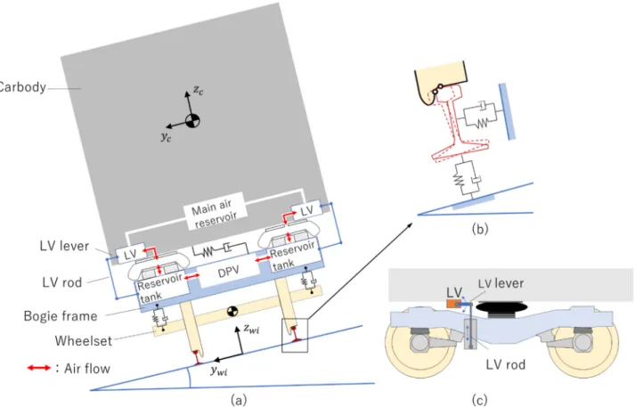
(2) Fig. 1 Railway vehicle model and coordinate systems: (a) rear view of vehicle components, (b) elastic wheel?rail contact model, and (c) side view of bogie with LV components. DPV: differential pressure valve; LV: levelling valve as follows: Awi = AcT Awi ,. Fig. 2. Vehicle motion description and coordinate systems (top view). of the origin of the wheelset trajectory coordinate system i can then be defined with respect to the moving carbody coordinate system as rwi � AcT ( Rwi � Rc ),. i � 1 4. (3). i = 1 4. (4). where Awi is the rotation matrix of the wheelset trajectory coordinate system with respect to the global coordinate system. The motion of the wheelset and bogie can be defined relative to the moving carbody reference coordinate system in this procedure. Therefore, simplifying assumptions for small relative displacements and rotations can be imposed in a straightforward manner when deriving the equations of motion, and this also leads to reduction of the computational cost in solving the governing equation. The degrees of freedom considered for the wheelset, bogie, and carbody models are summarized in Table 1. To determine the wheel and rail contact forces, a tabular contact search method is used to find contact points. Having determined contact points, the Hertzian normal contact force is defined with an elastic contact approach [5][6], while the Levi-Chartet’s nonlinear creep force model is used to define tangential forces in the contact patch. Contact forces are then dealt with as external forces in the governing equation. Table 1 Degree of freedom of the vehicle model. where Rc and Ac are, respectively, the global position vector and a rotation matrix of the moving carbody coordinate system, while Rwi is the global position vector of the wheelset trajectory coordinate system i. The rotation matrix of the wheelset trajectory coordinate system can also be written with respect to the moving carbody coordinate system 144. QR of RTRI, Vol. 62, No. 2, May 2021.

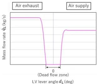
(3) 2.2 Thermodynamic air suspension system model In order to consider the nonlinearity and the airflow history of air spring system, we propose the coupling of a thermodynamic equation of air suspension system with the governing equations of vehicle motion given by (2). In the proposed air suspension system model, the air flow between reservoir tank, LVs, and DPVs are considered as shown in Fig. 3. An air spring is connected to a reservoir tank through an orifice. The spring is connected to a LV through a pipe to allow the air to flow in and out as needed. LV itself is attached to a carbody and the valve is opened and closed by a horizontal LV lever, which is connected to a bogie frame through a vertical LV rod, as shown in Fig. 1(c). That is, when a spring height dA, i.e., a relative distance between a carbody and bogie, decreases, the LV lever rotates to open the valve and compressive air is charged to the spring. The air is, on the other hand, discharged to the atmosphere when the spring height increases as the LV lever rotates in the opposite direction. The reservoir tanks of right and left springs are connected by a pipe through a DPV, as shown in Figs. 1 and 3. The air flow among the components shown in Fig. 3 are defined as follows: (a) Air spring-reservoir tank: qA (b) Air spring-LV: qL (c) Reservoir tank-DPV: qD With an assumption of polytropic process, the air spring pressure PA and the reservoir tank pressure PB can be obtained by PA P0 � ( � A � 0 )� , PB P0 � ( � B � 0 )�. LV mass flow rate ・qL is characterized as a function of the valve opening (i.e., LV lever angle) as shown in Fig. 4, where there is an airflow dead zone around the neutral LV lever angle. LV mass flow rate also depends on the upstream and downstream pressure, while the characteristic curve as Fig. 4 is obtained under certain conditions. Therefore, the characteristic curve is scaled based on the theoretical flow formula of compressive fluid, and LV flow rate of required condition in the numerical simulation is obtained. DPV mass flow rate ・qD is also obtained by similar procedures to that of LV flow rate.. Fig. 3 Airflow of air spring system model. DPV: differential pressure valve; LV: levelling valve. (5). where P0 and ρ0 are the air spring pressure and air density under the equilibrium condition, while ρA and ρB are the air density of the air spring and reservoir tank. κ is the polytropic index of the air. Using the law of mass conservation and (5), the air spring and reservoir pressure can be defined as a function of mass flows of the orifice, LV, and DPV as PA (q A , qL , d A ) � P0 PB (q A , qD ) � P0. �. �. � 0VA � q A � qL. � 0 �VA � � V ( d A ) � � V �q �q � 0 B. A. � 0VB. D. �. �, �. (6). where the volumes of the air spring and reservoir tank are given by VA and VB. δV(dA) defines a change in the air spring volume as a function of vertical spring deflection. The airflow rate in the orifice can be modelled by the following power function [7]: Rq A � � sign( PA � PB ) PA � PB. (7). where the exponent β and coefficient R are identified experimentally as described in the literature [7]. The vertical air spring force can then be defined as FAS � �( PA � Pat ) � Ae � � Ae (d A ) � � ( P0 � Pat ) Ae � FS. (8). where Pat is the atmospheric pressure, Ae is an effective area of the air spring, and δAe (dA) is the change of the effective area caused by vertical air spring deflection. FS is the vertical stopper force that is applied only if the air spring has the large deflection. The air spring forces given by (8) are applied to the carbody and the bogie, and added to the right hand side of (2). QR of RTRI, Vol. 62, No. 2, May 2021. Fig. 4 LV airflow rate characteristics 2.3 Coupled vehicle and air suspension system equation Using the flow rate equations for the air spring orifice, LV, and DPV, the air suspension system equations are defined in terms of their mass flow variables qA, qL, and qD as q A � g A (q A , qL , qD , d A ) � � q L � gL (q A , qL , d A , d L ) � q D � gD (q A , qD ) ��. (9). where dA and dL are the air spring deflection and the LV lever angle given from the vehicle model, respectively. Equation (9) can also be written in a compact form as follows: p = g( p, q ). (10). g g ] ,and q is the where p = [q q q ] , g = [ g generalized coordinate vector of a vehicle. Using (2) and (10), the governing equations for the coupled vehicle-air T A. T L. T T D. T A. T L. T T D. 145.

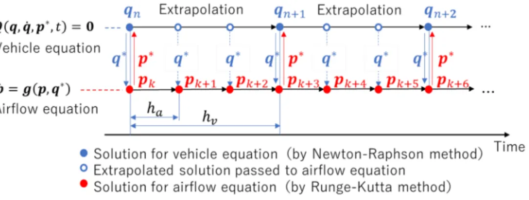
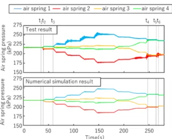
(4) suspension system model can be obtained as Q (q, q , p, t ) = 0 p = g( p, q ). (11). where the generalized force vector Q includes the air spring forces defined by the set of air suspension mass flow variables p. 3. Efficient solution procedure To solve governing equation (11), a co-simulation scheme was developed. The features of two equations in (11) can briefly be summarized as follows: (a) Vehicle equation: upper equation in (11) This equation is an ordinary differential equation in implicit form. Iterative convergence calculations are required to obtain the solution vector, while a large time step size in numerical calculation is allowed because of good convergence properties. (b) Air suspension equations: lower equation in (11) This equation is an ordinary differential equation in explicit form. A small-time step size is needed due to the nonlinearity of the air flow characteristics. However, since the dimensionality is small, computation cost is low even if explicit time integration is performed with a small time step size. Therefore, a co-simulation scheme is most suitable: where the two equations in (11) are solved in parallel while using optimal solvers for individual equations. A conceptual view of co-simulation scheme is shown in Fig. 5. The two calculating flows corresponding to each equation in (11) were defined, and solved by referring the solution of another flow (marked with an asterisk). Calculation time step sizes were set as ha and hv for vehicle and air flow equation, respectively. In this system, ha is defined as a smaller time step than hv. In addition, a variable time step was introduced in hv. When vehicles are running on a tangent track, a large step size is used to save computational cost as hv, while a small step is used during the transition curve to obtain accurate solutions. In order to solve the air flow equation, the vertical air spring deflection dA and LV lever angle dL, estimated by the solution of the vehicle equation at the same time, are required. Thus, an extrapolated position vector q* estimated by the solution of previous hv step was defined. The air flow equation was then solved by fourth order of Runge-Kutta method using dA and dL. estimated from q*. On the other hand, the vehicle equation was solved using the Newton-Raphson method with p* as the estimated air flow at the same time. The generalized velocity vector required to solve the vehicle equation was approximated using the following formula: qn �1 � 2(qn �1 � qn ) hv � qn. (12). The proposed co-simulation scheme leads to efficient solutions of the coupled system equations with low computational costs. 4. Numerical examples for the proposed method 4.1 Validation using stationary test results To validate the air suspension system model considering nonlinear LV airflow characteristics developed in this study, numerical simulation results were compared with results from a stationary test using a bogie rotational resistance testing machine, which can replicate the effect of the centrifugal force in curves as well. Relative yaw angle between bogie and carbody (bogie angle), and the centrifugal force exerted during curve negotiation are simulated by this stationary testing devices [1]. The testing scenario was as follows: (1) The bogie was rotated from 0 to 4 degrees (t1 - t2) (2) The lateral force simulating centrifugal force was applied to the carbody up to 20 kN/carbody, then, the applied force was released (t3 - t4) (3) The bogie was rotated from 4 to 0 degrees (t5 - t6) The numerical results from the proposed method were compared with test results in Fig. 6. Air springs on the front bogie were numbered as air springs 1 and 2, and those on the rear bogie as air springs 3 and 4, for the right and left sides. The motion of the LV lever angle observed in the test was well-reproduced in the numerical results, as shown in Fig. 6. Figure 6 also shows that the LV flow rate calculated in the numerical procedure was exhibited when LV lever angle exceeded the dead zone, as expected. The air pressure variation for the test and numerical results are shown in Fig. 7, and it can be confirmed that both results agree well. Through the validation, we conclude that the modeling of the air flow model is adequate, and the coupled motion of vehicle and the air suspension system could be well predicted using the proposed method. The computational time of dynamic numerical simulation, i.e., the procedure solving coupled equation of (1) and (10) by. Fig. 5 Co-simulation scheme for quasi-steady vehicle motion solver 146. QR of RTRI, Vol. 62, No. 2, May 2021.

(5) Fig. 6. Comparison of LV motion in stationary test scenario. of the dynamic numerical simulation in Fig. 8. The wheel load on the front axis of each bogie (No.1, No.3 axis) was estimated using each method assuming the vehicle was running on a curve of radius 160 m and a cant of 105 mm, at a speed of 10 km/h. The initial offset of LV lever angles within the dead zone were assumed so that the LV air flow occurred easily in this example: (1) Outer side of the front bogie and inner side of the rear bogie: initial LV lever angle shifted to the air supply side (2) Inner side of the front bogie and outer side of the rear bogie: initial LV lever angle shifted to the air discharge side. The load of the outer wheel was expected to be smaller than that of the inner wheel given the excess cant in this curve negotiation scenario. This tendency is reflected in Fig. 8, while the difference between inner and outer wheel load in the No.1 axis was smaller than that of No. 3 axis. This difference is caused by uneven LV airflow due to the initial offset. The air in the inner air spring of the front bogie tended to be discharged during the curve negotiation, decreasing air spring pressure. Therefore, the load of the inner wheels on the front bogie estimated using the proposed model was smaller than the estimations obtained by a model which does not consider LV air flow. Furthermore, it is shown in Fig. 8 that each wheel load was equal before entering the curve, while this was not the case after the curve negotiation and residual wheel load imbalance is exhibited. This phenomenon was well predicted with the proposed method as in the dynamic simulation. High-frequency variation of wheel load estimated in dynamic numerical result just after entering the transition curve cannot be seen in the proposed quasi-static method, while the computational times of a dynamic and the proposed simulations were 147 s and 7.0 s, respectively. This demonstrates a significant reduction in computational time with minimal loss in accuracy, as compared to the dynamic simulation model. To examine the LV-induced residual wheel load imbalance phenomenon, long-distance curve negotiation analysis was carried out using the proposed method to enable a quick. Fig. 7 Air spring pressure in stationary test scenario (Top: test, bottom: numerical simulation) numerical integration, was 72.2 s for the scenario as above, while that of proposed method was 5.4 s. It is confirmed from this result that the substantial reduction of computational cost is possible using proposed method. 4.2 Curve negotiation on the track In the next example, curve negotiation scenario is considered to validate the proposed method. The numerical results of the proposed method were compared with those QR of RTRI, Vol. 62, No. 2, May 2021. Fig. 8. Comparison of two simulation method for wheel load in single curve negotiation (Top: dynamics simulation, bottom: proposed method) 147.

(6) ulation schemes. The proposed procedure allows precise estimation of nominal vehicle motion in curves with less than 1/10 of computational time of the corresponding dynamics model. The proposed method therefore allows efficient numerical simulation for vehicle running scenarios over long distances. Numerical simulations for wear prediction of wheel and rail profiles as well as the air spring failure mode effect analysis for condition monitoring systems are potential applications in the future work. The proposed method will be improved further to account for non-Hertzian contact conditions between severely worn wheels and rails. References Fig. 9. Wheel load of No. 1 axis estimated by proposed method assuming long-distance running scenario. safety evaluation for practical use. About 20 km/h length of virtual track model were generated, which included 30 curves with a variety of curve radii and cants. The numerical simulation results of wheel loads on No.1 axis are shown in Fig. 9. The effect of the initial offset of the LV lever angle can be observed in Fig. 9: it shows that the wheel load imbalance gradually grew as the vehicle passed through multiple curves if an initial offset of LV lever angle was assumed. The computation times for this scenario were 3480 s and 80 s for the dynamic analysis and proposed simulation, respectively. It is thus possible to conclude that the proposed method allows us to perform running simulations over long distances efficiently while considering the history-dependent nonlinear air suspension behavior. 5. Conclusions An efficient and accurate numerical procedure taking into account the air flow history of an air suspension system for railway vehicle motion was developed in this study. Coupled governing equations for the quasi-static vehicle model and the thermodynamics air suspension model were developed. The equations were then solved through co-sim-. [1] Hondo, T. and Tanaka, T.,“Investigation of relationship between initial setting of leveling valves and air spring pressure of a railway vehicle when assuming the centrifugal force action,”Proceedings of the 26th IAVSD international symposium on dynamics of vehicles on roads and tracks, 2019. [2] Garg, V. and Dukkipati, R., Dynamics of railway vehicle, New York: Academic Press, 1984. [3] Tanaka, T. and Sugiyama, H.,“Prediction of railway wheel load unbalance induced by air suspension leveling valves using quasi-steady curve negotiation analysis procedure,”Proceedings of Institution of Mechanical Engineers, Part K, Vol. 234, No.1, pp.19-37, 2020. [4] Satou, E. and Miyamoto, M.,“Dynamics of a bogie with independently rotating wheels,”Vehicle System Dynamics, Vol.20, pp.519-534, 1992. [5] Shabana, A., Zaazaa, K. and Sugiyama, H., Railroad Vehicle Dynamics: A Computational Approach dynamics of railway vehicle, CRC Press, 2008. [6] Sugiyama, H., Sekiguchi, R., Matsumura, R., Yamashita, S. and Suda, Y.,“Wheel/Rail Contact Dynamics in Turnout Negotiations with Combined Nodal and NonConformal Contact Approach,”Multibody System Dynamics, Vol. 27, pp. 55-74, 2012. [7] Shimozawa, K. and Tohtake, T.,“An air spring model with non-linear damping for vertical motion,”Quarterly Report of RTRI, Vol. 49, pp.209-214, 2008.. Authors. . 148. Takayuki TANAKA, Ph.D.. Assistant Senior Researcher, Vehicle Mechanics Laboratory, Railway Dynamics Division Research Areas: Vehicle Dynamics, Running Safety Evaluation. . Hiroyuki SUGIYAMA, Ph.D.. Professor, Department of Mechanical Engineering, University of Iowa Research Areas: Computational Dynamics of Multibody Systems, Vehicle Dynamics. QR of RTRI, Vol. 62, No. 2, May 2021.

(7)