EMU’s Monetary and Fiscal Policy Effects on Euro Area Future Natural Interest Rate

EMU’s Monetary and Fiscal Policy Effects

on Euro Area Future Natural Interest Rate*

Hirotaka Suzuki

Freelance / Graduate of Graduate School of International Relations, University of Shizuoka E-mail: [email protected]

ABSTRACT

In this paper, we clarify whether monetary and fiscal policies, including those by consolidated governments such as by the European Union (EU), can affect the natural interest rate using New Keynesian models. First, when the modified New Keynesian Phillips curves are flat, we find that the Fisher equation easily holds empirically. However, the effects of monetary and fiscal policies, including those by consolidated governments such as the EU, on the natural interest rate are unclear. In contrast, when the modified New Keynesian Phillips curves are transitioning from being flat, the effectiveness of these policies on the natural interest rate increases. However, the Fisher equation is more difficult to hold empirically. Second, when the modified Intertemporal Substitution (IS) curves are not flat, these policies, as short-term nominal demand shocks, can affect the natural interest rate as the long-term equilibrium real interest rate. In contrast, when the modified IS curves become flat, although the short-term nominal monetary and fiscal policies are still effective, we possess limited or occasionally no effective ability of monetary and fiscal policies for affecting the natural interest rate. This is because the elasticity of these policies to the natural interest rate approaches zero.

Key words: Natural Interest Rate, New Keynesian Models, Modified Intertemporal Substitution

(IS) Curves, Modified New Keynesian Phillips Curves, Monetary and Fiscal Policies Including Consolidated Governments, The Fisher Equation, State-Space Model, Kalman Filter.

JEL Classification: E12, E43, E47, E52, E58, E63

* This paper is a revised version of a presentation at the 2018 EUSAAP Conference titled, “The Future of the EU and European Integration in the Aftermath of Crisis,” Section 5A “EU’s Monetary and Fiscal Policies” at the National Taiwan University, Taipei, 13:30–15:00, 29 June, 2018.

** I am grateful to 2 anonymous referees for their helpful comments and discussions as well as to the editor (Professor & Dr. Kentaro Iwatsubo, Kobe University) and the editorial board of JJMFE for their comments and patience during the process of resubmission.

1. Introduction

Recently, despite several ineffective policies and the implementation of unconventional and non-standard monetary policies of the European Central Bank (ECB), the European Union (EU) (or the (European) Economic and Monetary Union (EMU)) has seemingly escaped from deflation. The EU’s potential growth has slowed down to so called “Secular Stagnation” or long-term low growth. However, to date, the European causes of secular stagnation or low growth have not yet been empirically clarified. For Europe to have long-term, moderate real growth, an increase in the future potential growth or “natural interest rate” is required.

Borio, Disyatat, Juselius, and Rungcharoenkitkul (2017) show that monetary and fiscal policies may influence the natural interest rate, especially in the exceptional times of low interest rate after the European debt crisis. Further, verification of unconventional monetary policy effects on the natural interest rate has yet to gain much more research and scrutiny.

This paper aims to clarify the perspective of future EU growth potential by empirically focusing on monetary and fiscal policy effects of the EU member states on the natural interest rate. To assess the after-the-crisis growth potential, this paper takes into consideration the Wicksellian monetary policy regime (which incorporates the natural interest rate into the economic model) and Ricardian fiscal policy regime (which endows it to explicate causes of inflation expectation affecting natural interest rate). These weigh on monetary and fiscal fundamental deviations from equilibrium to explain future EU growth potential or natural interest rate momentum after the crisis.

1.1. Estimation of Natural Interest Rate and Filtering Algorithm Approach

Borio et al. (2017) explain that Keynes’ (1937) and Wicksell’s (1898) premise on capital market failure, as between the market and the natural rates, differs. Capital market failure is recognized as arbitrary by Keynes compared to appropriate by Wicksell. Afterwards, instead of Keynesian, New Keynesian ones as underlying friction are based on price stickiness.

Empirically, Holston, Laubach and Williams (2017) point out that measurements of natural interest rates have been more challenging because natural rates, like other latent variables, must be inferred from data. To do that, Holston, Laubach, and Williams (2017) and Justiniano and Primiceri (2010) estimate natural interest rates using the Kalman filter algorithm and based on the New Keynesian Phillips curves and Intertemporal Substitution (IS) curves.

Furthermore, Laubach and Williams (2015) explain that univariate time series methods such as the Hodrick–Prescott filter, the bandpass filter, and the unobserved components stochastic volatility model may be unreliable in periods when inflation and economic activity are not relatively stable. This is despite the argument that these methods could, in principle, work well at estimating the natural interest rate when inflation and economic activity are relatively stable.

Together, this indicates that real interest rates deviate from the natural rates for some time. However, the problem Laubach and Williams (2015) seek to point out are forward rates, including term premium. These factors contaminate the measurements of the market perception of the natural, short-term interest rate. They point out that movements in the term premium are a major source of variation in far-ahead forward rates. This means that forward rates are not a reliable measure of expectations of future interest rates.

To resolve this, Laubach and Williams (2015), instead of applying univariate time series methods to estimate the natural rate of interest use a multivariate Kalman filter that explicitly takes into account movements in inflation, output, and interest rates. The Laubach–Williams (LW) model treats the natural rate of interest as one that changes over time due to various influences. In the LW model, the natural rate is assumed to depend on the estimated contemporaneous trend growth rate of potential output and a time-varying unobserved component that captures the effects of other unspecified influences on the natural rate. We use this model with some modifications in our paper.

This paper is organized as follows. Section 2 presents the literature review. Section 3 constructs the economic models. Section 4 discusses the latent and unobserved variables in the model. Section 5 analyzes the observability conditions. Section 6 discusses the descriptive empirical methods. Section 7 presents the mathematical and statistical empirical methods. Section 8 describes the data. Section 9 presents the empirical results. Section 10 presents the conclusion of this paper.

2. Literature Review

Regarding the potential economic growth rate or natural interest rate, some research points out that lowering the population growth rate and population aging reduces the natural interest rate. Brand, Bielecki and Penalver (2018), and Fiorentini, Galesi, Pérez-Quirós, and Sentana (2018) present results on this idea as applied in Europe. Further, Fukuda (2017), and Iwata and Samikawa (2018) present results on this in Japan, mentioning that population decreases promote an increase in per capita capital and thereby lower the natural interest rate. Based on these contributions, we construct a modified New Keynesian economic model. We incorporate several stylized and seminal developments of the economic theory about these topics into this paper.

The original concept of the natural interest rate was first advocated by Wicksell (1898). Fisher (1930) incorporated the Euler equations of consumption into this model. Ramsey (1928) incorporated the determinant equations of population growth rate and natural interest rate into Wicksell’s original model. Following these developments, Woodford (2003) revived the concept of natural interest rate among academics and economic policy makers.

In estimating natural interest rate as latent or unobservable variables, the U.S. Federal Reserve’s economists Thomas Laubach and John C. Williams have been pioneers of the economic models of natural interest rate estimation from economic data. For example, Holston, Laubach, and Williams (2017) is their recent accomplishments.

Following these achievements, the New Keynesian economic model formulated forward-looking Euler equations of consumption, or GDP, into Wicksell’s model as IS curves. The New Keynesian economic model also formulated Forward-Looking nominal price rigidities and optimum price-setting mechanism of Calvo (1983) into the model as New Keynesian Phillips curves. The only issue is that these formulations cannot close the economic system, although the IS curves and New Keynesian Phillips curves are two important New Keynesian economic theoretical pillars. Therefore, we need further forward-looking (monetary and fiscal) policy rules influencing the GDP gap and inflation determination.

3. A Novel (and Modified) Forward-Looking New Keynesian Economic Model

This paper addresses these requirements by incorporating the modified Fisher equations and the modified Fiscal Theory of the Price Level (FTPL). The modified Fisher equations adjust nominal interest rate levels set by central banks to influence the natural interest rate under certain conditions. FTPL is modified by the double-entry system to solve the linearizing empirical specification problem of FTPL, and to concretely influence the natural interest rate in terms of both accumulated central government fiscal debt securities and equivalently private sector money stock as pointed out by Modern Monetary Theory (MMT). However, although the double-entry system is introduced to the model mainly by MMT, MMT itself does not necessarily lead to the following fiscal linear economic model specification if we accept only the credibility of the rules of the double-entry system. This closes the system of our proposed Forward-Looking New Keynesian economic model.

This paper analyzes the EU economy using the Forward-Looking New Keynesian state-space model including latent, unobservable variables, and observable variables. This is shown in the state transition equations and observation equations below. Both these equations consist of three types of terms: random walking unit-root processed and policy-effect-permanent real or latent terms that are often unobserved, stationary processed and policy-effect-transitory nominal terms that are observable, and error terms.

3.1. State-Space Model

The state-space model is defined as follows:

Y_t= Z_tX_t+ D_tW_t+ A_tu_t

X_t= T_tX_{t − 1}+ v_t

Here, Y_t: Observed variables, X_t: State or latent (unobserved) variables, W_t: Exogenous variables, Zt, Dt, At, Tt: Parameter matrix, ut, vt: Error terms.

In modeling a Forward-Looking New Keynesian economic model, this paper assumes equilibrium under the golden rule: IS rate (σt = 1), and household discount rate (ρt = 0).

3.2. Observed Equations

Observed V ariables_t= Permanent States_t+ Transitory Changes_t+ Error Terms_t

Observed equations comprise shock-effect-permanent latent, potential, and real unobserved variables, shock-effect-transitory observed stationary nominal variables, and error terms.

3.2.1. Modified IS Curves (Incorporating Population Growth Rate into the Model as GDP Per Capita Gap Rate) (y_t, r_t− r_t*):

y_t− n_t= E_ty_{t + 1}− E_tn_{t + 1}− i_t+ E_tπ_{t + 1}+ r_t* + { f }*ε_tyt − nt

n_t= n_t* + {l}*ε_tnt, 　　　 r_t= r_t* + {k}*ε_trt

y_t: GDP growth rate, n_t: Population growth rate, i_t: Nominal interest rate, π_t: Inflation rate, r_t:

Real interest rate, r_t*: Natural interest rate, n_t*: Potential population growth rate, ε_tyt − nt: Error term, ε_tnt: Error term, ε_trt: Error term

The modified IS curves are defined in such a way that the present term GDP gap rate (yt) is

determined by the coming term expected GDP gap (E_ty_t+1), the coming term expected inflation rate (Etπt+1), the nominal interest rate (it), and the natural interest rate (rt*). This incorporates the

population growth rate (nt) into GDP gap rate, which is modified as the (expected) GDP per

capita gap rate (E_ty_t+1 − E_tn_t+1 or y_t − n_t). The error terms of the observed equations (ε_tyt − nt, ε_tnt, ε_trt) are defined as stationary or constant terms, due to the monetary or fiscal policy implementation rules described below. Furthermore, if parameter {theta} = 1 and parameter {k} approaches zero, the modified IS curves become flat.

the current latent or unobserved real variables, and linearize them as E_ty_{t + 1}= y_t*, E_tn_{t + 1}= n_t*, and E_tπ_{t + 1}= π_t*. We linearize because directly modeling and estimating the coming term expected values in the state-space model causes problems of nonlinearity in estimating latent and unobserved variables. This allows us to deal with the estimation difficulty and empirical model specification. Economically and intuitively, because the effects of the present term latent and unobservable real values are persistent, it is natural for rational economic persons to regard them taken over to the next term as it is intact and unchanged, which is the rational expected value in the next term.

This is how we can let the transition equation be linear and it can be estimated using a Kalman filter (Kalman, 1960). The Kalman filter can only identify the latent or unobserved variables among the economic models composed of only linearized and simultaneous equations, including both observation equations and transition equations, meeting the appropriate observability conditions described in detail below.

3.2.2. Modified New Keynesian Phillips Curves (π_t, y_t− y_t*):

π_t = {al pha}*π_{t + 1}+ {beta}*y_t− {gamma}*y_t* − {delta}*n_t* + {theta}*r_t* − {ka p pa}*i_t

+{tau}*ε_tπt

n_t= n_t* + {l}*ε_tnt

Here, y_t*: Potential GDP growth rate, ε_tπt: Error term, and ε_tnt: Error term.

Modified New Keynesian Phillips curves posit that the present term inflation rate is determined by the next term expected GDP gap rate, the coming term expected inflation rate, the natural interest rate, the nominal interest rate, and the error terms. Similar to the modified IS curves, we incorporate population growth rate into the modified New Keynesian Phillips curves, which modify the GDP gap rate as GDP per capita gap rate. Likewise, we adopt the rational expectation theory in parameter estimation. Therefore, the coming term expected values are defined as the current term latent or unobserved real values to linearize the modified New Keynesian Phillips curves. Furthermore, modified New Keynesian Phillips curves become flat if both parameters {gamma} and {delta} approach zero.

3.2.3. Monetary Policy

Fisher Equation: rt = it − πt+1

Here, r_t: Real interest rate, i_t: Nominal interest rate, π_t+1: The next term inflation rate

3.2.3.1. The Fisher Equation’s Empirical Puzzle and Possibilities of Handling the Level of Natural Interest Rate

The Fisher equation is defined as the real interest rate equal to the nominal interest rate minus the expected inflation rate. Although the Fisher equation is reasonable in theory, the paradoxical and inexplicable empirical puzzle of Fisher equation comes out (as the cases of the misuse of natural interest rate instead of the real interest rate in Fisher equation are common in reality) if we mistakenly replace the real interest rate with the natural interest rate in the Fisher equation. Both are different concepts. The Fisher equation’s empirical puzzle is that if we have negative

coefficient ({k}) error terms in the natural interest rate specification (r_t = {z}*r_t* + {k}*ε_trt described as models below including components of financial regime with the coming term expectation terms not assumed in Fisher equation, and term premiums), we can see that the real interest rate and the natural interest rate respond to and move differently and adversely to each other, even with the same preconditions of their shocks and model specifications.

Concretely, the Fisher equation (it = rt + πt+1) indicates that with zero lower bound or with

negative nominal rate, if we fix nominal interest rate, raising the next term expected inflation rate causes real interest rate to decline. In contrast, if we fix the nominal interest rate, raising the coming term expected inflation rate causes the real interest rate to increase, with negative error

term {k} in i_t= {z}*r_t* + {k}*ε_trt+ π_{t + 1}. To put it in another way, it is not the rise of real interest rate but the rise of natural interest rate as the long-term equilibrium real interest rate. This is what we call the Fisher equation’s empirical puzzle.

To put the argument into shape, the Fisher equation (it = rt + πt+1) is represented as (expected future rates) + (real rates) = (nominal rates) for categorical classification.

Then, when we replace the real interest rate rt with its observation equation rt=

{z}*r_t* + {k}*ε_trt, we get i_t = {z}*r_t* + {k}*ε_trt+ π_{t + 1}. This indicates that the Fisher equation (i_t= {z}*r_t* + {k}*ε_trt+ π_{t + 1}) is classified as (expected future rates) − (real equilibrium rates)

= (nominal rates). This is because when {k}*ε_trt is negative, we have empirical cases of r_t* > 0 as well as rt < 0, which is contradictory to the empirically paradoxical case to (the misuse of) the

theory of Fisher equation (i_t = r_t + π_t+1) with (i_t= {z}*r_t* + {k}*ε_trt+ π_{t + 1}). That is, if we misuse the short-term real interest rate with the natural interest rate as the long-term equilibrium real

interest rate (however, this misuse often happens in reality), empirical analysis of the theory of

Fisher equation reveals that the negative error term {k}*ε_trt occasionally causes a real interest rate to move against and adversely to the direction indicated by the Fisher equation.

As causes of negative error term {k}*ε_trt, we can mention the cases of the inflation targeting regime in Japan and in Europe in deflation. In the inflation targeting regime of Japan, raising the

coming term expected inflation rate means declining real interest rate, which equals {k}*ε_trt becoming negative in r_t= {z}*r_t* + {k}*ε_trt with real interest rate not directly influencing the natural interest rate. At this stage, we do not discuss whether changes in real interest rate affect changes in the natural interest rate (we discuss this matter later, though). As this is one of the

examples, we can also look at other reasons for negative error terms {k}*ε_trt.

The discrepancy between the real interest rate and the natural interest rate indicates that under certain circumstances, central banks (including consolidated governments) can take both real

interest rate and natural interest rate to their targeted levels through the error term {k}*ε_trt as short-term nominal demand shocks by implementing fiscal and monetary policies. We focus on the conditions below, which can lead the natural interest rate level to the targeted levels to some degree by utilizing specific monetary and fiscal policies.

3.2.3.2. Arguments about Conditions for Leading the Natural Interest Rate to Targeted Levels

r_t = {z}*r_t* + {k}*ε_trt

In the observation equation r_t, we let the parameter {z} be intact or unrestricted whether it is in a unit root process (or non-stationary process) or a stationary process. This is because the restriction on it embraces the matter about its determinacy of different and important policy

implications compared to each other. Here, r_t*: Natural interest rate and ε_trt: Error term

First, in the observed equation of real interest rate r_t, policy shocks {k}*ε_trt of real interest rate

rt never affect the natural interest rate rt* structurally, with parameter {z} = 1. That is, the natural

interest rate r_t* is in the unit root process to real interest rate rt, or the natural interest rate rt* is a

random walk to real interest rate r_t.

We have the parameter {z ≠ 0, 1} below, which indicates that the natural interest rate r_t* is not a random walk to the real interest rate rt. It also indicates that there is some relationship between

interest rate r_t* except for the random walk or unit root process. To consider this, we apply the pure expectations hypothesis below to connect the short-term real interest rate with the natural interest rate.

3.2.3.3. Pure Expectations Hypothesis

r_t* = 1_n

∑

t = 0 n

r_t+ χ_t

where, 1_n∑_{t = 0}n r_t in general is not a random walk of r_t to r_t*.

When we have 1_n∑_{t = 0}n r_t= r_t, we obtain the relation r_t= r_t* − χ_t.

Here, r_t*: Natural interest rate as the long-term equilibrium real interest rate expiring in the n-term, r_t: Short-term real interest rate expiring in the next term, and χ_t: Term premium.

In the pure expectations hypothesis, the long-term equilibrium real interest rate r_t* is defined

as the average sum of the short-term ranges of the short-term real interest rate 1_n∑_{t = 0}n r_t plus term

premium χt. Therefore, when we have 1_n∑t = 0n rt = rt, the natural interest rate as the long-term

equilibrium real interest rate r_t* is defined as the average short-term real interest rate rt plus term

premium χt. The larger the degrees of uncertainty in the economic circumstances and

expectations about future economies, the larger the term premium χ_t becomes. In addition, the term premium χt is usually non-zero in reality. For the monetary policy scope of the changes in

the term premium χ_t, central banks’ monetary easing policy, such as quantitative easing (QE), could reduce the term premium χt to a lesser extent with more uncertain economic conditions.

The pure expectations hypothesis allows the observation equation r_t to affect the natural interest rate as a long-term equilibrium real interest rate by causing policy-driven shocks to short-term real interest rate, due to the specific relations set among natural interest rates and real interest rates. This is different from the case with a random walk ({z} = 1).

In concrete terms, when we put the pure expectations hypothesis into the observation equation

rt, we obtain rt* − χt={z}*rt* + {k}*εtrt. By solving this problem, we obtain 1 − z rt* =

χ_t+ {k}*ε_trt. If were rearrange it, we get r_t* = _{1 − z}1 χ_t+ _{1 − z}k ε_trt. This means that only when parameter {z} is not in unit root (z ≠ 1) and parameter {k} is not zero (k ≠ 0), both the term premium and policy-driven shocks to the real interest rate, including the inflation target regime, can affect the natural interest rate as the long-term equilibrium real interest rate through multiplier effects.

expectations hypothesis into the observation equation r_t, so that we can obtain r_t* =

i_t+_{1 − z}1 χ_t+ _{1 − z}k ε_trt− π_{t + 1}. According to the Fisher equation, the rise of nominal interest rate i_t and term premium χt raises the natural interest rate rt*. However, when the short-term policy

shock term _{1 − z}k ε_trt gets negative and is large, the Fisher equation may possibly not hold in reality and empirically. Thereafter, we verify it in the empirical part of the paper.

However, we then introduce fiscal policy and have further arrangements about causes of inflation expectation, focusing on the expectation term −π_t+1 modified by fiscal policy. To put the results in advance, when we consider consolidated governments, we can modify the inflation

expectation term as −π_{t + 1}= − s_{t + 1}* + s_{t + 1}− m_{t + 1}− { j}*ε_tst. Thus, we can finally obtain the equation for the natural interest rate determination as r* = i_{t t}+ _{1 − z}1 χ_t+_{1 − z}k ε_trt− s_{t + 1}* + s_{t + 1}−

m_{t + 1}− { j}*ε_tst.

3.2.3.4. Implications of Monetary Policy Driven Error Terms Becoming Zero r_t− r_t* = 0

When central banks always set monetary policies as r_t= r_t* in all periods, error terms emanating from nominal rigidities become zero, consequently closing both the output gap

y_t− y_t* and inflation gap π_t− π_t* at a time. This condition is called the Divine coincidence. Central banks respond to these gaps by arranging policy interest rates, and then by tightening or easing the business cycles depending on economic circumstances. Thus, when these gaps are zero, the economic system stabilizes.

However, monetary policies are less effective than fiscal policy in increasing money stocks (or the accumulation of private sector surpluses) of private sector economic agents instead of monetary bases. This is because central banks basically supply monetary bases, not money stocks, to private banks by lending with repayment according to the interest rate imposed by central banks or exchange government securities held by central banks with money stock held by private banks.

By the way, with parameter {theta} = 1, the modified IS curve gets flatter with parameter {k} approaching to zero.

3.2.4. Fiscal Policy

3.2.4.1. Equations of Private Sector Surplus Rate with MMT Based on the Rules of Bookkeeping by Double Entry

Δ Private Sector Sur plus Rate

Consolidated Government Net M oney Stock Issued Rate _t

= Central Government De f icits Rate G_t− Tax_{t t} +Current Account Balance Sur plus Rate Ex_t− Im_{t t}

With the rules of bookkeeping by double entry, the private sector surplus rate is defined as the central government deficit rate plus current account balance surplus rate. When the central government’s fiscal position is in equilibrium, the private sector balance sheet has a net surplus only when the current account balance is in net surplus. On the other hand, when the overseas sector is in equilibrium, the private sector balance sheet has a net surplus only when the private sector gets to hold all the new government securities just issued by the central government (or all the money stocks newly issued by the central bank), both of which are the same in terms of consolidated government balance sheets. That is, the sum of newly issued central government securities is the same quantity as the sum of the newly issued money stock issued by the central bank.

3.2.4.2. Modified Price Equations Based on MMT and FTPL

s_t= s_t* + m_t− π_t+ { j}*ε_tst

Here, s_t: Private sector surplus (money stock held by private sector) growth rate, s_t*: Potential private sector surplus (potential money stock held by private sector) growth rate, π_t: Inflation

rate, ε_tst: Error term, mt: Money stock growth rate

Based on FTPL from Watanabe and Iwamura (2004) and Iwamura (2018), the price equation

(s_t= s_t* + m_t− π_t+ { j}*ε_tst) is derived by the model described below. FTPL: Π_t = M t + Bt − It

St + Rt

Here, Π_t: Price level, M_t: Money stock volume, B_t: Aggregate government security issued volume, St: Expected government credit creation issued volume, It: Private financial institution’s

lending volume, R_t: Consolidated central government reserves volume

In FTPL, price levels are determined as the ratio of the sum of consolidated central government liabilities (M_t + B_t − I_t) to the sum of consolidated central government assets

(S_t + R_t): Π_t= M t + Bt − It

St + Rt .

Then, compared to the scale of the consolidated central government’s issued money stock held by private sectors, the volumes of both private financial institution’s lending I_t and consolidated central government reserves Rt are negligible in scale to other variables’ volumes. Thus, when

we set It = 0, Rt = 0, we obtain Πt = M t + Bt_St . Then, we log-linearize Πt= M t + Bt_St , so that we get

lnΠ_t = ln(M_t + B_t) − lnS_t. In this transformation, we can do that only with the rules of bookkeeping by double entry, which MMT supports. Of course it is not one of the peculiar features of MMT. As MMT pointed out from the fact of bookkeeping by double entry, we can get

Mt = Bt because both sides of the balance sheet of the consolidated central governments are the

same. This means that the sum of the issued central government securities is the same as the sum of the issued money stocks held by private sectors. Consequently, when we differentiate lnΠt =

ln(Mt + Bt) − lnSt with (Mt = Bt), we obtain Π˙t_Πt = 2M˙ _t 2M t −

S˙t

St, so that we have a transitory policy

shock term s_ttransitory= m_t− π_t. Then, when we incorporate it into the observation equation st, we

obtain s_t= s_t* + m_t− π_t+ { j}*ε_tst, with {j} = 1. This means the random walk of the error term of the short-term nominal private sector surplus rate ε_tst because of the non-existence of reasonable convergence fiscal policy target levels of short-term nominal private surplus rate.

When we transform it as one term ahead, we obtain −π_{t + 1}= − s_{t + 1}* + s_{t + 1}− m_{t + 1}− { j}*ε_{t + 1}st . Then, we incorporate −π_{t + 1}= − s_{t + 1}* + s_{t + 1}− m_{t + 1}− { j}*ε_{t + 1}st into the natural interest rate equation r_t* = i_t+ _{1 − z}1 χ_t+ _{1 − z}k ε_trt− π_{t + 1} we derived in previous section on monetary policy, so that we finally obtain r_t* = i_t+ _{1 − z}1 χ_t+ _{1 − z}k ε_trt− s_{t + 1}* + s_{t + 1}− m_{t + 1}− { j}*ε_{t + 1}st . This indicates that in terms of fiscal policy, a permanent rise in the private sector surplus growth rate declines the natural interest rate, and that a transitory increase in private sector surplus raises the natural interest rate. Furthermore, it shows that an increase in the supplied money stock growth rate held by the private sector issued by the consolidated central government reduces the natural interest rate. We verify this with the EU economy in the empirical part of the paper.

4. Latent Variables

Latent variables equations are defined in permanent shock terms, transitory shock terms, and error terms as described below.

State V ariables_t*

= Permanent States State V ariables_{t − 1}* + Transitory Changes_{t − 1}+ Error Terms_t

This paper defines transitions of latent variables as unit root processed permanent random walk (including growth and non-growth factors) plus error terms. Non-growth factors are defined as all the mixed factors excluding both growth factor and the defined factors in the models below. 4.1. Transition Equations y_t* = y_{t − 1}* + s_{t − 1}* + g_{t − 1}yt* + ε_tyt* s_t* = s_{t − 1}* + g_{t − 1}st* + ε_tst* π_t* = π_{t − 1}* + y_{t − 1}* − n_{t − 1}* + g_{t − 1}πt* + ε_tπt* r_t* = r_{t − 1}* + y_{t − 1}* − n_{t − 1}* + g_{t − 1}rt* + ε_trt* n_t* = n_{t − 1}* + y_{t − 1}* + g_{t − 1}nt* + ε_tnt*

g_tyt*= {a}*g_{t − 1}yt* + ε_tgt

yt* , g_tst*= {b}*g_{t − 1}st* + ε_tgt st* g_tπt*= {c}*g_{t − 1}πt* + ε_tgt πt* , g_trt*= {d}*g_{t − 1}rt* + ε_tgt rt* g_tnt*= {e}*g_{t − 1}nt* + ε_tgt nt*

Here, y_t*: Potential GDP growth rate s_t*: Potential real private sector surplus (private-sector held money stock) growth rate π_t*: Potential inflation rate r_t*: Natural interest rate n_t*: Potential

population growth rate y_t* − n_t*: Potential GDP per capita growth rate g_tyt*: Contribution of non-growth factors to potential GDP non-growth rate (%) g_tst*: Contribution of non-growth factors to potential real private sector surplus (private-sector held money stock) growth rate (%) g_tπt*: Contribution of non-growth factors to potential inflation rate (%) g_trt*: Contribution of non-growth factors to natural interest rate (%) g_tnt*: Contribution of non-growth factors to potential population growth rate (%) ε_t: Error terms

Although we have already defined both observable and latent variables so far, we still need to define and meet the requisite model identification conditions to verify the model empirically. We discuss the identification conditions of the empirical model in the following subsections.

4.2. State-Space Model Y_t= Z_tX_t+ D_tW_t+ A_tu_t X_t= T_tX_{t − 1}+ v_t 4.3. Observation Equations Y_t= y_t s_t π_t r_t n_t = Z_tX_t+D_tW_t+ A_tu_t = 1 0 1 1 0 1 0 0 −1 0 0 0 0 0 0 0 0 0 0 0 −γ 0 α θ −δ 0 0 0 0 0 0 0 0 z 0 0 0 0 0 0 1 0 0 0 0 0 0 0 0 0 ∙ y_t* s_t* π_t* r_t* n_t* g_tyt* g_tst* g_tπt* g_trt* g_tnt* + 0 0 0 −1 0 0 1 0 0 0 0 1 −1 0 0 0 β 0 0 0 0 0 −κ 0 0 0 0 0 0 0 0 0 0 0 0 0 0 0 0 0 ∙ y_t s_t π_t r_t n_t m_t i_t π_{t + 1} + f 0 0 j 0 0 0 0 0 0 0 0 τ 0 0 0 0 0 0 0 0 k 0 0 l ∙ ε_tyt − nt ε_tst ε_tπt ε_trt ε_tnt

4.4. Transition Equations X_t= T_tX_{t − 1}+ v_t y_t* s_t* π_t* r_t* n_t* g_tyt* g_tst* g_tπt* g_trt* g_tnt* = 1 1 0 0 1 0 1 0 1 0 0 0 0 0 −1 1 0 0 1 0 0 1 −1 0 1 1 0 0 1 0 0 0 0 0 0 0 0 1 0 0 0 0 0 0 0 1 0 0 0 1 0 0 0 0 0 0 0 0 0 0 0 0 0 0 0 0 0 0 0 0 0 0 0 0 0 a 0 0 b 0 0 0 0 0 0 0 0 0 0 0 0 c 0 0 0 d 0 0 0 e ∙ y_{t − 1}* s_{t − 1}* π_{t − 1}* r_{t − 1}* n_{t − 1}* g_{t − 1}yt* g_{t − 1}st* g_{t − 1}πt* g_{t − 1}rt* g_{t − 1}nt* + ε_tyt* ε_tst* ε_tπt* ε_trt* ε_tnt* ε_tgt yt* ε_tgt st* ε_tgt πt* ε_tgt rt* ε_tgt nt*

Taking the empirical results in advance, we have a = 1.036506***, b = 0.8486726***, and c = d = e = 0. Thus, with just rank η = 7, all the state variables in the state-space model are all observable and identifiable.

O = Z ZT ZT2 ZT3 ⋮ ZT η − 1 = y_t s_t π_t r_t n_t =

2 ∙ 1 T η − 1, 1T η − 1, 0 1T η − 1, 1 T η − 1, 0 1 T η − 1, 2 ∙ −1 T η − 1− 1T η − 1 0 0 −γ + α + θ − δ 1T η − 1, −γ 1 T η − 1, α 1 T η − 1, 1 T η − 1, α + θ −1 T η − 1− δ 1 T η − 1 z 1T η − 1 0 1 T η − 1 0 0 0 z 1 T η − 1 z −1 T η − 1 0 1 T η − 1 5. Observability Conditions

With empirical analysis, we can exactly define observability (or identification) conditions to verify whether the state-space model described above has justly identified latent variables utilizing all the observed variables in the model.

O = Z ZT ZT2 ZT3 ⋮ ZT η − 1 = rank η

Only with O = rank η, the state variables are identified. This defines all the state variables exactly estimated.

With flat modified IS curves or with flat modified New Keynesian Phillips curves, the identification problems of latent variables estimation uncertainty come out, causing impossibility of simply estimating or specifying all latent variables in the state-space model, including both potential growth factors and non-growth factors from all the observable variables in the equations.

However, when we let state variable gaps be stationary, which assumes the error term convergence of observation equations, the identification problems of flat modified IS curves or flat modified New Keynesian Phillips curves are resolved. Intuitively, its restriction is natural and rational because New Keynesian utilizes fiscal and monetary policies to close the gaps. Furthermore, when the gaps are completely closed by New Keynesian fiscal and monetary policies, the economic system stabilizes the most.

With these identification problems, a model cannot identify those unobservable latent variables. The characteristics of justly identifiable conditions consisting of the models and

observed variables on parameters and latent variables transitions is called Observability, which was introduced by Kalman (1960). In a time-invariant linear system, the observability of the models can be verified by checking the ranks of the observability matrix. Furthermore, as additional identifying restrictions, imposing observable variables allows for the decomposition of both permanent and non-stationary real latent variables and both transitory and stationary gaps, helping meet the observability restrictions. That is why even with flat modified IS curves or flat modified New Keynesian Phillips curves, the results of empirical analysis of the models in this paper meet observability restrictions and are more robust.

The observation equation π_t could be the same as those of the observation equations y_t and r_t, under specific parameter value sets of πt, in which case the models cannot be identifiable.

Furthermore, the observed equations y_t, π_t, and r_t possess two potential inherent equations to materialize. Without resolving these possibilities, the models cannot meet observability conditions O = rank η (in this case, we have O > rank η). Therefore, we consider the following specific cases and derive identification conditions for verifying criteria in estimating parameters and latent variables in the models.

5.1. Observability Conditions: Two Unidentifiable Cases

Unidentifiable Case 1: The Case with a Zero GDP gap of Observed Equation y_t= π_t y_t= y_t* .

y_t = y_t* means that in the equation Nominal GDP Growth Rate = Real GDP Growth Rate + Inflation Rate, it leads to Real GDP Growth Rate = 0. This indicates that the economy is in equilibrium. In economic equilibrium, model identifications are impossible, as latent variables in the models become zero. In this case, both modified IS curves and modified New Keynesian Phillips curves are identical.

From the identical equation of y_t = π_t, we have the unidentifiable simultaneous conditions of −γ + α + θ − δ = 2, −γ = 1, α = 1, (α + θ) = 2, and −δ = 1, which require γ = −1, α = 1, θ = 1, and

δ = 1 simultaneously. This means that all terms like the π_t* (Potential inflation rate), y_t* − n_t*

(Potential GDP per capita growth rate), and r_t* (Natural interest rate) are in unit root processes. This indicates that the changes of those latent variables obey random walk with the duration of the changes being permanent. In addition, with y_t* = 0, the model itself is unidentifiable.

Unidentifiable Case 2: The Case with coincidence of interest rates of savings and investments

under full employments of observation equations π_t= r_t r_t = r_t* (Also, the case with term premium χt = 0 of the pure expectations hypothesis rt= rt* − χt)

In this case, the observation equations of πt and rt are identical simultaneously. This indicates

that in addition to the random walk of the changes in inflation rate, we have the problems of flat modified IS curves and/or flat modified New Keynesian Phillips curves. The flat curves make

the identification of the parameters and latent variables of the model much harder.

From the identical equations of πt = rt, we have unidentifiable conditions with −γ + α + θ − δ =

z, −γ = 0, α = 0, α + θ = z, and −δ = 0 simultaneously, which needs to meet z = 1, γ = 0, α = 0, θ =

1, and δ = 0 at the same time. This means that the changes from term (t) to term (t + 1) of only r_t* (Natural interest rate) are in random walk with the duration of the changes being permanent.

In this case, although the gap variables (inflation gaps and GDP gap) are not zero, the parameters of the modified IS curves and modified New Keynesian Phillips curves are completely flat.

The modified and flat IS curves mean that output gaps y_t− y_t* are never or hardly responsive to changes in past real interest rate gaps r_t− r_t* . It also means that we have the case with the term premium χ_t = 0 of the pure expectations hypothesis r_t= r_t* − χ_t.

The modified and flat New Keynesian Phillips curves are defined as cases with inflation rates never or hardly responsive to changes in past output gaps. Here, the modified New Keynesian Phillips curves are flat with the parameter γ = 0, and δ = 0. Meanwhile, we have the modified IS curves flat or flatter, when we have {z} = {θ} = 1 and {k} = 0, or {k} approaching and close to 0, in the observed equation of r_t (Real interest rate).

Taking the empirical results in advance, we consider the least possibility of {z} = 1. Indeed, we have z = 0.0041854*** at the 1% significance level. Furthermore, we have {k} relatively close to zero (k = 0.2423523***), which indicates that modified IS curves may not be flat. On the other hand, remembering that with γ = 0 and δ = 0, the modified New Keynesian Phillips curves would be flat. Indeed, we have γ = 0.0032266** and δ = 0.0039947*, which may be verified as flat modified New Keynesian Phillips curves with relatively high probability due to the significance levels of the results.

Unless we meet even one of the two unidentifiable cases described above (y_t ≠ π_t ≠ r_t), the state-space models of the paper are assured of being identifiable. To take in advance the empirical results of the parameter estimation, we can be assured of those identifications because the parameters do not meet the unidentifiable conditions above.

6. Empirical Methods and Assumptions

6.1. Why Is the State-Space Model Appropriate for Estimating Natural Interest Rate?

In the real world, both measurable “observable values” and unobservable “state or latent variables” are present. The state-space model estimates the unobservable states or latent variables by using “observable values” and “state or latent variables.” In terms of directly unobservable ones, the natural interest rate, which is the main theme of the paper, is estimated by

the state-space model as one of the general economic models that deals with the issue successfully.

Economic models or equations derived from economic theories have employed the state-space model in empirical analysis. This is because the state-space model directly incorporates unobservable latent variables into the models. In many cases, these economic models can be stylized in the form of a state-space model or equations. Therefore, in estimating natural interest rate, such as that in this paper, utilizing the state-space model for both theoretical and empirical analysis is not only a requisite but also feasible.

Although the modified New Keynesian model of this paper has incorporated several unobservable real variables, including the natural interest rate, into the model, making those in stylized forms as a state-space model resolves the problems to estimate those latent variables empirically. In addition, the empirical analysis of the modified New Keynesian model is feasible, utilizing measurable “observable values” to estimate unobservable latent variables both rationally and efficiently from the models.

The state-space model allows the economic model to incorporate not only directly unobservable latent variables, such as natural interest rate, but also other observable macro explanatory variables into the model. For example, the modified New Keynesian model here allows all measurable GDP growth rates, population growth rates, nominal interest rates, inflation rates, and real interest rates to more or less influence the determination of unobservable natural interest rate.

This paper utilizes a multivariate (diffuse) Kalman filtering approach to estimate the natural interest rate, which takes several observed explanatory variables into consideration. From a theoretical perspective, the univariate filtering approach can be used to estimate the natural interest rate, such as filtering the short-term real interest rate to estimate the natural interest rate. However, the modified New Keynesian model assumes several economic equations within the models to estimate the natural interest rate. Consequently, in estimating the natural interest rate, expanding the range of incorporating possible explanatory variables into the modified New Keynesian models is meaningful in terms of economic or public policy implications such as verifications of stylized academic works, including economic theories and empirical analyses.

As concrete methods of the Kalman filter, the state-space model has two types of inherent equations: “observation equations” and “transition equations.” Observation equations are those that obtain observed values from latent values. Transition equations obtain the next term state values from the present term state values. This paper stylizes these “observation equations” and “transition equations” in the models from the modified New Keynesian models described above.

6.2. Foundations of Kalman Filter v_t= Y_t− Z_tX_t− D_tW_t P_t= H_tH_t′ F_t= Z_tP_tZ_t′ + A_tA_t′ K_t= T_tP_tZ_t′ + A_t F_t−1 X_{t + 1}= T_tX_t+ K_t Y_t− Z_tX_t− D_tW_t P_{t + 1} = T_t− K_tZ_t P_tT_t′ + H_t− K_tA_t H_t′ = T_tP_tT_t′ + H_tH_t′ − K_t{ T_tP_tZ_t′ + H_tA_t′ } = T_tP_tT_t′ + P_t− K_tF_tK′_t

6.3. What Is Kalman Filter?

In the state-space model, the algorithm that effectively estimates the coming term unobserved latent variables such as natural interest rate from the present term state or latent variables is called the Kalman filter. The Kalman filter needs to obtain the noise of both observed variables and latent or state variables to correct the estimates of state or latent variables. Methodologically, we need to estimate the noise variances of both “observation equations” and “transition equations” by the Maximum Likelihood Method (or MCMC by Bayesian Simulation, which we do not discuss in the paper, though). In maximizing the likelihood, the Kalman filter is also involved in its process.

The Kalman filter deals with two tasks. First, it forecasts the next term state or latent estimated forecast values from the present term state or latent estimated values, utilizing the present term observed values. Second, with the present term observed values, it corrects the present term state or latent variable estimated values.

The processes of the Kalman filter correction of the estimated values are described below.

Corrected States

= Pre Corrected States + Kalman Gain ×

　Realized Observed V alues − Estimated Observed V alues

When observed variables and latent or state variables are not correlated with each other so much, the noises of observation equations are defined to be large. This shows that the realized observed variables are not useful to estimate the state or latent variables at the time. In contrast, when the present term state or latent variables do not coincide with the next term state or latent variables, the noises of transition equations are regarded as large. This means that the present

term estimated state or latent values are not so helpful in estimating the coming term state or latent values. Therefore, with larger discrepancies among realized observed values and estimated observed values, the scales of the Kalman filtering correction become larger. Consequently, Kalman Gains are defined as follows.

Kalman Gain = Forecast Error V ariances o f States

÷ Forecast Error V ariances o f States +V ariances o f Observation Equation Noises

In addition, the forecast error variances of states are calculated as follows.

The Next Term Forecast Error V ariances o f States

　= The Present Term Forecast Error V ariances o f States +V ariances o f Transition Equation Noises

Once we obtain realized observed values, the forecast error variances of states become smaller. In Kalman filter, considering “realized observed values,” it corrects “the next term forecast error variances of states” and we obtain the following.

Corrected Forecast Error V ariances o f States

　= 1 − Kalman Gain × PreCorrected Forecast Error V ariances o f States

Furthermore, the Kalman gain never becomes larger than 1.

Here, we have explained the state-space model and Kalman filter as theoretical and intuitive foundations. Now, we proceed to explain their rigorous mathematical and empirical foundations.

7. Mathematical and Statistical Foundations of State-Space Model and Kalman Filter (Mainly Based on Francke, Koopman and de Vos (2010) and De Jong (1991))

Using Francke, Koopman, and de Vos (2010), we expand the models by De Jong (1991) in detail below. We have observation equations and transition equations with several assumptions.

Observation Equation: Y_t = Z_tX_t + D_tW_t + A_tu_t

Transition Equation: Xt = TtXt−1 + vt

Assumptions: The error terms are assumed to be zero mean, normally distributed, serially uncorrelated, and uncorrelated with each other: vt~N(0, σ2Q), ut~N(0, σ2H), E vtv′ = 0 for alls

Furthermore, we have a scaling factor, σ, and variance matrix, Q and H, depending on the vector of nuisance parameters ω, which makes the parameter Θ a Diffuse Random Vector below. Considering ω, we have u_t~N(0, σ2_{Ω), which we write as Ω = Ω(ω), X}

t = Xt(ω), Wt = Wt(ω). ω

represents all other factors that have effects on the variables of the model and can be estimated empirically.

We let ζ: Dimension of time series vector y, ϕ: Number of vectors of coefficient Θ, μ: μ = ζ −

ϕ, which is the ζ × μ dimension of the transformation matrix J_t.

The state-space model estimates the parameters of the linear state-space models by maximum likelihood. The diffuse Kalman filter is a method for recursively obtaining linear, least squares forecasts of Yt conditional on past information. These forecasts are used to construct the diffused

log likelihood when the model is nonstationary. When the model is stationary, we utilize the Kalman filter instead.

7.1. State-Space Model Initial State Vector

We have the initial conditions of the state vector X1 below.

X₁= ι + ΘΓ + ξC, 　Θ N 0, σ2∑ 　ξ N 0, σ2Q₀

Here, ι: Vector; Γ, C, Q0: Fixed system variables of appropriate dimensions; ξ: Random vector

independent of the other disturbances; Θ: Fixed and unknown diffuse random vector.

Based on the value of X1, the state-space model estimates the coming term of X1, utilizing the

(Diffuse) Kalman filter below.

7.2. Diffused Log-Likelihood of State-Space Model

We obtain general diffused likelihood functions that can be utilized and analyzed invariant to the nuisance term ω as follow.

logLD=𝓁_∞* y; σ, ω = lim Σ−1 0 𝓁 y; σ, ω +1 2log 2πσ 2_Σ 𝓁 y; σ, ω = 𝓁 y Θ; σ, ω + 𝓁 Θ; σ, ω − 𝓁 Θ y; σ, ω −2𝓁 y Θ; σ, ω = −2𝓁 y; Θ, σ, ω

= ζ log2π + ζ logσ2+ log F_t + σ−2 Y_t− Z_tX_t− D_tW_t ′

F_t−1 Y_t− Z_tX_t− D_tW_t

−2_{𝓁 Θ y; σ, ω}

= ϕlog2π + ϕlogσ2− log Σ−1+ W_t′F_tW_t

+σ−2Θ′ Σ−1+ W_t′F_t−1W_t Θ

+σ−2 Y_t− Z_tX_t− D_tW_t ′F_t−1W_t Σ−1 +W_t′F_t−1W_t −1W_t′F_t−1 Y_t− Z_tX_t− D_tW_t

−2σ−2 Y_t− Z_tX_t− D_tW_t ′F_t−1W_tΘ

So, we get −2𝓁 y; σ, ω = ζlog2π + ζlogσ2+ log F_t + log Σ + log Σ−1+ W_t′F_tW_t +

σ−2 Y_t− Z_tX_t− D_tW_t ′ F_t−1− F_t−1W_t Σ−1+ W_t′F_t−1W_t −1W_t′F−1_t Y_t− Z_tX_t− D_tW_t

The diffuse log-likelihood functions are as follows.

−2logLD= − 2_𝓁∞ y; σ, ω = ζ log2π + ζ logσ2+ log F_t + log W_t′F_t−1W_t + σ−2RSS

Maximizing −2logLD= −2_𝓁∞(y; σ, ω) about parameter σ2_{, we obtain the following.}

−2logL_cD= −2_𝓁∞ y; σ, ω = ζ log2π + ζ logRSS − ζ logn + log F_t + log W_t′F_t−1W_t + ζ So, we get logLD=_𝓁∞* y; σ, ω = lim

Σ−1 0

𝓁 y; σ, ω + 12log 2πσ2Σ .

7.3. Marginal Log-Likelihood of the State-Space Model

Why do we need marginal log-likelihood instead of diffuse log-likelihood? If we have nuisance ω and parameter vectors Θ, we must estimate and analyze them by utilizing the marginal log-likelihood below. Although the diffuse log-likelihood is not necessarily invariant to the nuisance parameter ω, the marginal log-likelihood in this paper is always invariant to ω, when ω is linearly dependent on Wt (that is, Wt = Wt (ω)), which is needed to analyze them with

nuisance parameter ω.

To transform diffused ones into marginal ones, we let y* = Jt y. Jt does not depend on either Θ

or ω. Furthermore, we have J_t′W_t= 0, which means J_t ′ and W_t are not correlated at all. Third, we replace ζ with μ, and obtain the full rank Jt. Finally, we let Jt*′Jt* and Wt′Wt be proportional to

each other: J_t*′J_t* _{∝ Wt}′W_t.

Then, the marginal log likelihood functions are obtained as follows.

−2𝓁 y*, σ, ω =

As J_t′W_t = 0, J_t J_t′F_tJ_t −1J_t′ = F_t−1M_F

　　　　　　　　where M_F = I − W_t W_t′F−1_t W_t −1W_tF_t−1

Therefore, J_t′F_tJ_t = F_t ∙ J_t′J_t ∙ W_t′W_t−1∙ W_t′F_t−1W_t

As J_t′J_t = 1, the marginal log-likelihood functions are defined as follows.

−2logLM = −2𝓁 y*, σ, ω

= μlog2π + μlogσ2+ log F_t + log W_t′F_t−1W_t − log W_t′W_t + σ2RSS

Maximizing −2logLM = −2_{𝓁(y*, σ, ω) about parameter σ}2_{, we obtain the following.}

−2logL_cM = −2_{𝓁 y*, σ, ω}

= μlog2π + μlogRSS − μlogm + log F_t + log W_t′F_t−1W_t − log W_t′W_t + μ

7.4. Evaluation of Diffused and Marginal Log-Likelihood

In evaluating diffused log-likelihood, we evaluate it using the methods below.

RSS = q − s′S−1s, 　　q =

∑

∑

∑

The maximizations of the diffused log-likelihood about parameter Θ, σ2 _{are shown as follows.}

Θ = S−1s, σ2= q − s′S−1s /σ2

On the other hand, in order to obtain marginal log-likelihood, with J_t*′J_t* _{∝ Wt}′W_t, we transform S, V, J into terms as defined below, maximizing the marginal log-likelihood about parameter Θ and σ2_{, and estimate them.}

V_t* = Z_tJ_t* + D_tW_t J_{t + 1}* = T_tJ_t* v* = L Y_t− Z_tJ_t* − D_tW_t S* = W_t′W_t=

∑

∑

∑

∑

Θ* = S* − 1s*, σ2*= q* − s*′S* − 1s* /σ2

We employ these methods and procedures to estimate the parameters Θ and diffuse Kalman filter.

8. Data Description

All the observed variables utilized and analyzed in this paper are listed and explained in detail below. All variables are in percent-change compared with the same period in the previous year.

y: GDP growth (%). Seasonally and calendar-adjusted data, at current prices, in million euro (from Eurostat).

n: Total population growth, national concept (%). Unadjusted data (i.e. neither seasonally adjusted nor calendar-adjusted data), thousand persons (from Eurostat)

π: HICP (%). Overall index excluding energy and unprocessed food index, 2015 = 100 (from Eurostat).

i: EONIA (%) (from ECB statistical data warehouse).

m: M3 growth (%) (from ECB statistical data warehouse) [million euro].

g-t: Net financial transactions (%), Liabilities, STK_FLOW central government consolidated, in million euro, total economy and rest of the world (from Eurostat).

ex-im: Current account growth (%). Financial account, net positions at the end of period to rest of the world, in million euro (from Eurostat).

s: (g-t) + (ex-im) private saving growth (%).

Data ranges of time series economic data in the Euro area are uniformly set from 2008Q1 to 2019Q2 (from the global financial crisis to the present) because we conform them to the variable whose availability length is the shortest of all.

9. Empirical Results

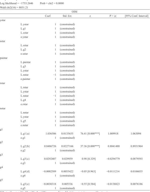
9.1. Modified New Keynesian Phillips Curves Are Flat and Modified IS Curves Are Not Flat

The estimation results are shown in Table 1 and Table 2. We evaluate the New Keynesian Model using the results of these two tables.

Against the conditions of {z} = 1, {k} ≈ 0. This allows the modified IS curves to be flat or not. Consider the least possible outcome of {z} = 1. Indeed, we have {z} = 0.0041854*** at the 1% significance level. Furthermore, we have {k} relatively closer to zero ({k} = 0.2423523***) as in case 2. Therefore, we may infer that the modified IS curves may not be flat.

In contrast, we have flat, modified New Keynesian Phillips curves. Remember that with γ = 0 and δ = 0, the modified New Keynesian Phillips curves would be flat. Indeed, we have γ =

0.0032266** (significant at 5% level) and δ = 0.0039947* (significant at 10% level). This can be inferred as the existence of flat modified New Keynesian Phillips curves.

Depending on the results of parameter estimation whether modified IS curves and modified Table 1 Empirical Results of State-Space Model-1

Sample: 2009q1 - 2019q2 Number of obs = 42 Log likelihood = −1753.2646 Prob > chi2 = 0.0000 Wald chi2(16) = 8031.21

OIM

Coef. Std. Err. z P > |z| [95% Conf. Interval] ystar L.ystar 1 (constrained) L.g1 1 (constrained) L.sstar 1 (constrained) e.ystar 1 (constrained) sstar L.sstar 1 (constrained) L.g2 1 (constrained) e.sstar 1 (constrained) paistar L.paistar 1 (constrained) L.g3 1 (constrained) L.ystar 1 (constrained) L.nstar −1 (constrained) e.paistar 1 (constrained) rstar L.rstar 1 (constrained) L.ystar 1 (constrained) L.nstar −1 (constrained) L.g4 1 (constrained) e.rstar 1 (constrained) nstar L.nstar 1 (constrained) L.ystar 1 (constrained) L.g5 1 (constrained) e.nstar 1 (constrained) g1 L.g1{a} 1.036506 0.0135655 76.41 [0.000***] 1.009918 1.063094 e.g1 1 (constrained) g2 L.g2{b} 0.8486726 0.0227166 37.36 [0.000***] 0.8041488 0.8931964 e.g2 1 (constrained) g3 L.g3{c} 0.0292407 0.029959 0.98 [0.329] −0.0294779 0.0879593 e.g3 1 (constrained) g4 L.g4{d} −0.0002589 0.0055422 −0.05 [0.963] −0.0111214 0.0106035 e.g4 1 (constrained) g5 L.g5{e} −0.0030318 0.005536 −0.55 [0.584] −0.0138823 0.0078186 e.g5 1 (constrained)

*** significant at 1%, ** at 5%, * at 10%. Note: Model is not stationary. (Continue) Source: Author

New Keynesian Phillips curves are flat or not, we have various potential results on natural interest rate determination. Furthermore, we incorporate both natural interest rate and fiscal and monetary policies, including those by consolidated governments, into the Fisher equation. Therefore, we can scrutinize the relationship between the Fisher equation and natural interest rate.

9.2. The Less Flat Modified New Keynesian Phillips Curves Become, the Less Realized the Fisher Equation Holds

According to the simulation results constructed by economic models and empirical analysis of this paper, we have confirmed the so-called Fisher equation’s empirical puzzle, which does not identify and empirically holds the Fisher equation (Figure 1), as discussed earlier in section 3, when with short-term nominal demand shock term reacting elastically to the economy ({k} > 1) (or when the elasticity of short-term demand shocks are relatively large (k ≠ 1 and k ≈ 1)). This means that Fisher’ s empirical puzzle gets realized relatively easily, when the economy is not in

Table 2 Empirical Results of State-Space Model-2

OIM

Coef. Std. Err. z P > |z| [95% Conf. Interval] GDP ystar 1 (constrained) nstar −1 (constrained) paistar 1 (constrained) rstar 1 (constrained) Population 1 (constrained) InterestRate −1 (constrained) e.GDP{f} −140.9696 23.73586 −5.94 [0.000***] −187.491 −94.44815 Inflation paistar{alpha} −0.0001234 0.0004897 −0.25 [0.801] −0.0010833 0.0008364 ystar{gamma} 0.0032266 0.0015567 2.07 [0.038**] 0.0001756 0.0062777 nstar{delta} 0.0039947 0.0021505 1.86 [0.063*] −0.0002201 0.0082096 rstar{theta} −0.0050515 0.0007992 −6.32 [0.000***] −0.0066179 −0.0034852 InterestRate{kappa} 0.5589732 0.1046738 5.34 [0.000***] 0.3538162 0.7641302 GDP{beta} −0.0722508 0.0204628 −3.53 [0.000***] −0.112357 −0.0321445 e.Inflation{tau} −0.1573956 0.0226896 −6.94 [0.000***] −0.2018664 −0.1129247 PricvateSectorSurplus sstar 1 (constrained) MoneyStock 1 (constrained) Inflation −1 (constrained) e.PricvateSectorSurplus{j} 1 (constrained) RealInterestRate rstar{z} 0.0041854 0.0006486 6.45 [0.000***] 0.0029141 0.0054566 e.RealInterestRate{k} 0.2423523 0.0359976 6.73 [0.000***] 0.1717983 0.3129064 Population nstar 1 (constrained) e.Population{l} 21.97505 2.837119 7.75 [0.000***] 16.4144 27.5357 *** significant at 1%, ** at 5%, * at 10%. Note: Model is not stationary.