Fukuoka Institute of Technology
Graduate School of Engineering
Implementation of Simulation Systems and
Testbed for WMNs: Simulation and Experimental
Results
by
Tetsuya ODA
Adviser: Prof. Leonard Barolli
i
Contents
List of Figures vii
List of Tables viii
Acknowledgement ix
Abstract x
Chapter 1 Introduction 1
1.1 Background . . . 1
1.2 Research Goal . . . 2
1.3 Research Interests and Related Work . . . 2
1.4 Thesis Contribution . . . 3
1.5 The Structure of The Thesis . . . 4
Chapter 2 Wireless Networks 5 2.1 Wireless Network Introduction . . . 5
2.2 Wireless Architecture . . . 5 2.2.1 Infrastracture Architecture . . . 5 2.2.2 Ad Hoc Architecture . . . 6 2.3 Wireless vs. Wired . . . 6 2.3.1 Collision . . . 7 2.3.2 Unidirectional Links . . . 7 2.3.3 Asymmetric Links . . . 7
2.4 The Wireless Channel . . . 7
2.4.1 The Free Space Propagation Model . . . 8
2.4.2 The Two-Ray Ground Model . . . 8
2.4.3 The Shadowing Model . . . 9
2.5 Overview of DCF and EDCA Protocols . . . 10
2.5.1 Distributed Coordination Function (DCF) . . . 10
2.5.2 Enhanced Distributed Channel Access (EDCA) . . . 11
2.6 Ad Hoc Routing Protocols . . . 11
2.6.1 Reactive Routing . . . 12
2.6.2 Proactive Routing . . . 13
Contents
2.7 Mobile Ad-hoc Networks (MANETs) . . . 17
2.8 Vehicular Ad-hoc Network (VANET) . . . 18
2.9 Wireless Sensor and Actor Networks (WSANs) . . . 18
2.9.1 WSAN Architectures . . . 18
2.9.2 WSAN Challenges . . . 18
2.10 Internet of Things (IoT) . . . 19
2.11 Ambient Intelligence (AmI) . . . 19
Chapter 3 Wireless Mesh Networks 21 3.1 Introduction to WMNs . . . 21 3.2 Architectures of WMNs . . . 22 3.3 Application Scenarios of WMNs . . . 23 3.4 WMNs Evaluation Techniques . . . 24 3.4.1 Simulations . . . 24 3.4.2 Emulators . . . 25 3.4.3 Real-World Testbeds . . . 25
Chapter 4 Intelligent Algorithms 26 4.1 Introduction to Intelligent Algorithms . . . 26
4.2 Genetic Algorithm . . . 30
4.3 Tabu Search . . . 31
4.4 Hill Climbing . . . 31
4.5 Simulated Annealing . . . 32
Chapter 5 Genetic Algorithms 33 5.1 Introduction to Genetic Algorithms . . . 33
5.2 The Appeal of Evolution . . . 34
5.3 Elements of Genetic Algorithms . . . 35
5.4 A Simple Genetic Algorithm . . . 36
5.5 Some Applications of Genetic Algorithms . . . 36
Chapter 6 Simulation Systems Implementation 38 6.1 Introduction to Mesh Router Node Placement Optimization . . . 38
6.2 Node Placement Problems and Their Applicability to WMNs . . . 39
6.3 Optimization Problems . . . 40
6.4 Ad hoc Methods for Mesh Router Nodes Placement . . . 43
6.5 Neighborhood Search-based Algorithms . . . 44
6.6 WMN-GA System . . . 45 6.7 WMN-TS System . . . 49 6.8 WMN-HC System . . . 50 6.9 WMN-SA System . . . 52 6.10 Web Interface . . . 53 6.11 ns-3 . . . 55 ii Tetsuya ODA
Contents
Chapter 7 Simulation Results 57
7.1 Simulation Scenario 1 . . . 57
7.1.1 Simulation Description and Design . . . 57
7.1.2 Discussion of Simulation Results . . . 59
7.2 Simulation Scenario 2 . . . 63
7.2.1 Positioning of Mesh Routers by WMN-GA . . . 64
7.2.2 Simulation Description . . . 66
7.2.3 Discussion of Simulation Results . . . 68
7.3 Simulation Scenario 3 . . . 70
7.3.1 Simulation Settings . . . 70
7.3.2 Discussion of Simulation Results . . . 72
7.4 Simulation Scenario 4 . . . 74
7.4.1 Simulation Settings . . . 74
7.4.2 Simulation Results . . . 76
7.5 Simulation Scenario 5 . . . 78
7.5.1 Simulation Settings . . . 78
7.5.2 Discussion of Simulation Scenario . . . 82
Chapter 8 Testbed Implementation 87 8.1 Testbed Design and Implementation . . . 87
8.1.1 Description . . . 87
8.1.2 Testbed Interface . . . 88
8.1.3 Testbed Environment . . . 89
8.2 Experimental Environment . . . 89
Chapter 9 Experimental Results 92 9.1 Experimental Scenario 1 . . . 92
9.1.1 Scenario Description . . . 92
9.1.2 Experimental Results . . . 94
9.1.2.1 Experimental Settings and Parameters . . . 94
9.1.2.2 Experimental Measurements . . . 94
9.2 Experimental Scenario 2 . . . 94
9.2.1 Scenario Description . . . 94
9.2.2 Experimental Results . . . 95
9.2.2.1 Experimental Settings and Parameters . . . 95
9.2.2.2 Experimental Measurements . . . 96
9.3 Experimental Scenario 3 . . . 97
9.3.1 Scenario Description . . . 97
9.3.2 Experimental Results . . . 97
9.3.2.1 Experimental Settings and Parameters . . . 97
9.3.2.2 Experimental Measurements . . . 97
Contents
9.4.1 WMN Testbed for Distributed Concurrent Processing . . . 100
9.4.1.1 Open MPI . . . 100
9.4.1.2 NAS Parallel Benchmarks . . . 100
9.4.2 Scenario Description . . . 100
9.4.3 Experimental Results . . . 101
9.4.3.1 Experimental Settings and Parameters . . . 101
9.4.3.2 Experimental Measurements . . . 103
Chapter 10 Conclusions and Future Work 105 10.1 Conclusions . . . 105
10.1.1 Conclusions from Simulation Results . . . 105
10.1.1.1 Simulation Scenario 1 . . . 105
10.1.1.2 Simulation Scenario 2 . . . 106
10.1.1.3 Simulation scenario 3 . . . 107
10.1.1.4 Simulation scenario 4 . . . 107
10.1.1.5 Simulation scenario 5 . . . 107
10.1.2 Conclusions from Experimental Results . . . 108
10.1.2.1 Experimental Scenario 1 . . . 108 10.1.2.2 Experimental Scenario 2 . . . 108 10.1.2.3 Experimental Scenario 3 . . . 109 10.1.2.4 Experimental Scenario 4 . . . 109 10.2 Future Work . . . 109 References 109 References 110 List of Papers 116 iv Tetsuya ODA
v
List of Figures
1.1 The structure of the thesis. . . 3
2.1 Ad-Hoc and infrastructure mode. . . 6
2.2 Two-ray Ground Propagation Model. . . 9
2.3 MPRs selection, reaching all 2-hop neighbors . . . 14
2.4 Configuration process of HWMP. . . 16
6.1 Cross Region Crossover. . . 47
6.2 Mutation operators. . . 49
6.3 System structure for Web interface . . . 54
6.4 Web interfaces . . . 54
7.1 Simulation results of the WMN-GA for Uniform distribution. . . 59
7.2 Simulation results of the WMN-TS for Uniform distribution. . . 60
7.3 Simulation results of the WMN-HC for Uniform distribution. . . 60
7.4 Simulation results of the WMN-SA for Uniform distribution. . . 60
7.5 Simulation results of the WMN-GA for Normal distribution. . . 61
7.6 Simulation results of the WMN-TS for Normal distribution. . . 61
7.7 Simulation results of the WMN-HC for Normal distribution. . . 61
7.8 Simulation results of the WMN-SA for Normal distribution. . . 62
7.9 Simulation results of the WMN-GA for Exponential distribution. . . 62
7.10 Simulation results of the WMN-TS for Exponential distribution. . . 62
7.11 Simulation results of the WMN-HC for Exponential distribution. . . 63
7.12 Simulation results of the WMN-SA for Exponential distribution. . . 63
7.13 Simulation results of the WMN-GA for Weibull distribution. . . 63
7.14 Simulation results of the WMN-TS for Weibull distribution. . . 64
7.15 Simulation results of the WMN-HC for Weibull distribution. . . 64
7.16 Simulation results of the WMN-SA for Weibull distribution. . . 64
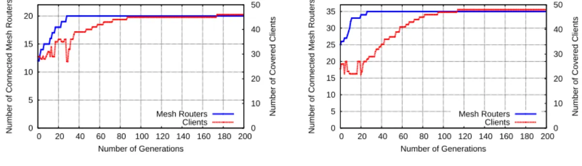
7.17 SGC and NCMC vs. number of generations for Normal distribution. . . 65
7.18 SGC and NCMC vs. number of generations for Uniform distribution. . . 65
7.19 SGC and NCMC vs. number of generations for Exponential distribution. . . 66
7.20 SGC and NCMC vs. number of generations for Weibull distribution. . . 66
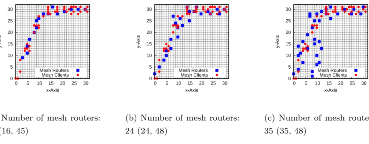
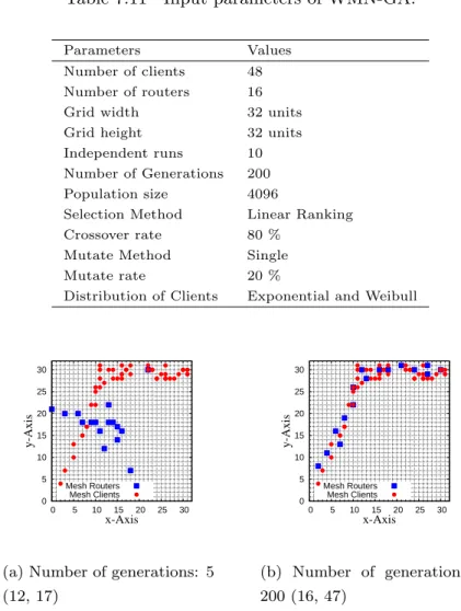
7.21 (m, n): m is SGC, n is NCMC for Normal distribution. . . . 67
List of Figures
7.23 (m, n): m is SGC, n is NCMC for Exponential distribution. . . . 67
7.24 (m, n): m is SGC, n is NCMC for Weibull distribution. . . . 68
7.25 Results of mean PDR. . . 69
7.26 Results of mean throughput. . . 70
7.27 Results of mean delay. . . 71
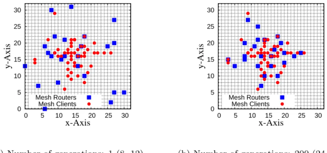
7.28 (m, n): m is SGC, n is NCMC (Exponential distribution). . . . 72
7.29 (m, n): m is SGC, n is NCMC (Weibull distribution). . . . 72
7.30 Results of average PDR for no. of generations 200. . . 73
7.31 Results of average throughput for no. of generations 200. . . 73
7.32 Results of average delay for no. of generations 200. . . 74
7.33 (m, n): m is SGC, n is NCMC for normal distribution. . . . 75
7.34 SGC and NCMC vs. number of generations for normal distribution. . . 76
7.35 Results of average throughput. . . 77
7.36 Results of average delay. . . 77
7.37 Results of average jitter. . . 77
7.38 Results of fairness index. . . 78
7.39 (m, n): m is SGC, n is NCMC of normal distribution. . . . 79
7.40 (m, n): m is SGC n is NCMC of uniform distribution. . . . 79
7.41 (m, n): m is SGC, n is NCMC (Exponential distribution). . . . 79
7.42 (m, n): m is SGC, n is NCMC (Weibull distribution). . . . 80
7.43 SGC and NCM vs. number of generations for Normal Distribution. . . 80
7.44 SGC and NCM vs. number of generations for Uniform Distribution. . . 80
7.45 SGC and NCM vs. number of generations for Exponential Distribution. . . 81
7.46 SGC and NCM vs. number of generations for Weibull Distribution. . . 81
7.47 Results of average throughput for WMNs using HWMP of different distributions. 83 7.48 Results of average delay for WMNs using HWMP of different distributions. . . . 83
7.49 Results of remaining energies for WMNs using HWMP of different distributions. . 84
7.50 Results of average throughput for WMNs using OLSR of different distributions. . 85
7.51 Results of average delay for WMNs using OLSR of different distributions. . . 85
7.52 Results of remaining energies for WMNs using OLSR of different distributions. . 86
8.1 Snapshot of the testbed. . . 88
8.2 Testbed interface. . . 88
8.3 Experimental environment for scenario 1. . . 89
8.4 Experimental environment for scenario 2. . . 90
8.5 Experimental environment for scenario 3. . . 90
8.6 Experimental environment for scenario 4. . . 91
9.1 Snapshot of nodes in the testbed for scenario 1. . . 93
9.2 Experimental results for 1→ 5. . . . 95
9.3 Snapshot of nodes in the testbed for scenario 2. . . 96
9.4 Experimental results for 1→ 5. . . . 98
9.5 Snapshot of nodes in the testbed for scenario 3. . . 99
9.6 Experimental results for 1→ 5. . . 101
9.7 Snapshot of nodes in the testbed for scenario 4. . . 102
viii
List of Tables
2.1 Values of the path loss exponent in different environments. . . 10
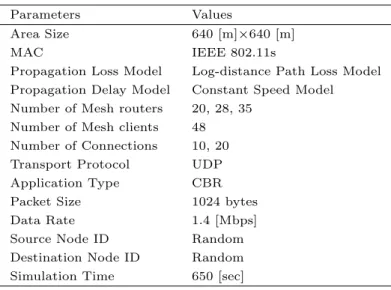
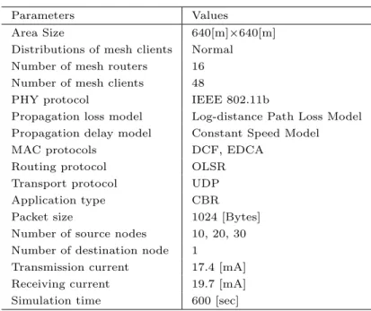
7.1 Input parameters of WMN-GA. . . 57
7.2 Input parameters of WMN-TS. . . 58
7.3 Input parameters of WMN-HC. . . 58
7.4 Input parameters of WMN-SA. . . 58
7.5 The p-value of SGC of Friedman test. . . 59
7.6 The p-value of NCMC of Friedman test. . . 59
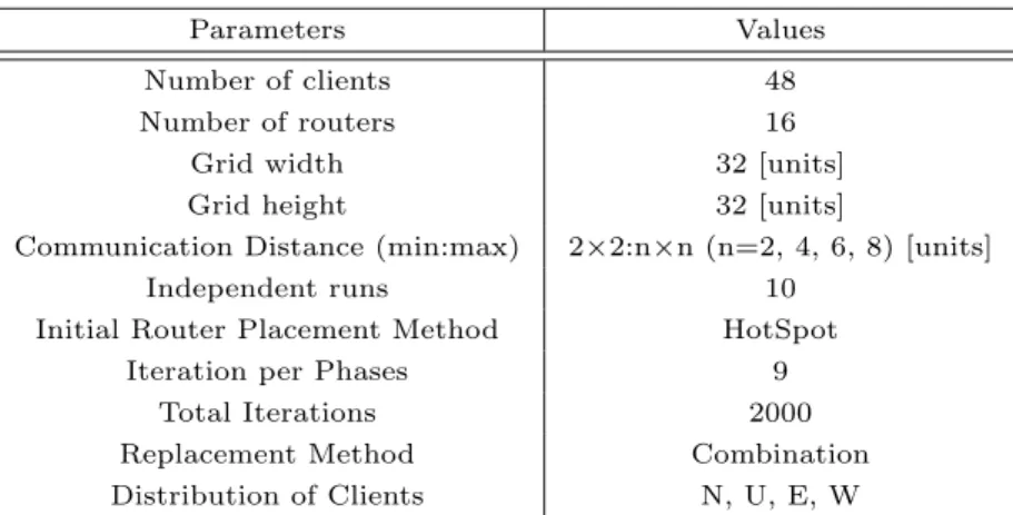
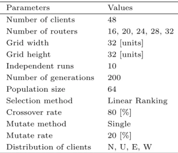
7.7 Input parameters of WMN-GA. . . 65
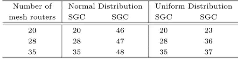
7.8 Evaluation of WMN-GA for Normal and Uniform distributions. . . 66
7.9 Evaluation of WMN-GA for Exponential and Weibull distributions. . . 66
7.10 Simulation parameters. . . 68
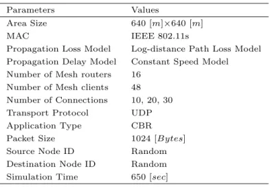
7.11 Input parameters of WMN-GA. . . 72
7.12 Simulation parameters. . . 73
7.13 Input parameters of WMN-GA system. . . 75
7.14 Evaluation of WMN-GA system. . . 75
7.15 Simulation parameters for ns-3. . . 76
7.16 Input parameters of WMN-GA system. . . 78
7.17 Evaluation results of WMN-GA system. . . 81
7.18 Simulation parameters for ns-3. . . 82
9.1 Experimental parameters for scenario 1. . . 92
9.2 OLSRd parameters. . . 92
9.3 Experimental parameters for scenario 2. . . 97
9.4 Experimental parameters for scenario 3. . . 100
9.5 Experimental parameters for scenario 4. . . 103
ix
Acknowledgement
Working three years to complete my Ph.D. course was not an easy task. The help of many professors and colleagues was needed. First, I would like to thank my advisor Professor Leonard Barolli, for his continuous efforts and support during these six years. He was always ready to listen and to advice my ideas. He taught me how to be practical and persistent in my research without giving up.
I would like to give special thanks to Professor Shigeto Nishida, Dr. Makoto Ikeda and Professor Shijie Zhu as members of inspection committee. They gave me very good advices and suggestion to improve the quality of my thesis.
I thank Professor Kazunori Uchida and Professor Jiro Iwashige, for their comments and support. I also thank Professor Fatos Xhafa for his long talks and innovative ideas in my research field. A special thank goes to Professor Makoto Takizawa and Professor Tomoya Enokido, who always supported me spiritually and gave a lot of feedback in my presentations. I would like to thank also Dr. Keita Matsuo, Dr. Tao Yang, Dr. Elis Kulla, Dr. Evjola Spaho and Dr. Masahiro Hiyama for their kind support, advices and friendship.
My research in Fukuoka Institute of Technology was also inspired by all members of INA labora-tory. I thank all students of INA Laboratory studying for many hours in the laboratory, inspiring me to work harder.
Finally I would like to thank my parents, Toyofumi and Chiemi, my brother Kenta, for their spiritual support. Therefore, I want to dedicate this thesis to my beloved family. Their educational support is priceless.
x
Abstract
A Wireless Mesh Network (WMN) can be defined as a collection of mobile nodes, which form a highly resource constrained network and a dynamic topology. Because of the dynamic topology, routing procedures and protocols are a key field of testing and research. In a research environment, research tools are required to test, verify and identify problems of an algorithm or protocol. These tools are classified in three major techniques: simulators, emulators and real-world testbeds. In most of research in WMNs, their performance is evaluated in both quantitative and qualitative aspects. Throughput performance, routing efficiency, energy consumption are some of the key issues that are addressed frequently on WMNs. The WMN technology has to ensure a certain degree of security and scalability and provide the infrastructure for distributed collaborative computing.
In this thesis, we design and implement simulation systems and a testbed in order to analyse the performance of different routing protocols, architectures, OSs, queue management algorithms and mobility models. From the evaluation results, we found that the mobility of nodes brings oscillations in performance and route instabilities. We found that multiple flows traffic decreases the performance of the network.
The contributions of our work are: 1) implementation and evaluation of a different meta-heuristics methods for mesh router node placement; 2) implementation of a simulation tool for WMNs using NS3; 3) implementation and evaluation of a Raspberry Pi based WMN testbed; 4) application of WMN testbed in real environments, considering different scenarios; 5) evaluation of WMN testbed in different OSs; 6) evaluation of WMN testbed considering distributed concurrent processing; 7) our research work give insights about future developments and integration of WMNs as an important technology of wireless communication.
The outline of the thesis is as follows. In Chapter 1 is shown the background and the motivation of the thesis. In Chapter 2, we introduce general aspects of wireless networks. We discuss wireless architectures and wireless technologies giving advantages and disadvantages for each of them. We present WMNs in Chapter 3. We discuss problems of WMNs and describe the routing protocols and their features. In Chapter 4, we introduce general aspects of meta-heuristics methods. We present Genetic Algorithms (Gas), Tabu Search (TS), Hill Climbing (HC) and Simulated Annealing (SA). We show in details the GA and its operators in Chapter 5. The simulation systems are presented in Chapter 6. We give details of radio propagation models, mobility models and other parameters. Then, we show different scenarios and the traffic data that we used for simulations. In Chapter 7, we introduce the implemented testbed. We give details of technical and environment settings. Then we show the experimental scenarios. In Chapter 8 and Chapter 9, we discuss the results of the simulations and experiments, respectively. Chapter 10 concludes the thesis. We present some concluding remarks and future work.
1
Chapter 1
Introduction
1.1
Background
Wireless Mesh Networks (WMNs) can be seen as a special type of wireless ad-hoc networks. WMNs are based on mesh topology, in which every node (representing a server) is connected through wireless links to one or more nodes, enabling thus the information transmission in more than one path. The path redundancy is a robust feature of mesh topology. Compared to other topologies, mesh topology does not need a central node, allowing networks based on it to be self-healing. These characteristics of networks with mesh topology make them very reliable and robust networks to potential server node failures.
There are a number of application scenarios for which the use of WMNs is a very good alternative to offer connectivity at a low cost. It should also mentioned that there are applications of WMNs which are not supported directly by other types of wireless networks such as cellular networks, ad hoc networks, wireless sensor networks and standard IEEE 802.11 networks. There are many applications of WMNs in Neighboring Community Networks, Corporative Networks, Metropoli-tan Area Networks, Transportation Systems, Automatic Control Buildings, Medical and Health Systems, Surveillance and so on.
There are a lot of works done on testbed for WMN and Mobile Ad-hoc Network (MANET). In [1], the authors analyze the performance of an outdoor ad-hoc network, but their study is limited to reactive protocols such as Ad hoc On Demand Distance Vector (AODV) and Dynamic Source Routing (DSR). The authors of [2] perform outdoor experiments of non standard pro-active protocols. Other ad-hoc experiments are limited to identify MAC problems, by providing insights on the one-hop MAC dynamics as shown in [3].
In [4], the authors present an experimental comparison of OLSR using the standard hysteresis routing metric and the Expected Transmission Count (ETX) metric in a 7 by 7 grid of closely spaced Wi-Fi nodes to obtain more realistic results. The throughput results are similar to our previous work and are effected by hop distance [5]. In [6], the authors did not care about the routing protocol. In [7], the disadvantage of using hysteresis routing metric is presented through simulation and indoor measurements.
Also, there are some other research works done for WMNs. In [8], the authors present the architecture, security, and management of SwanMesh. The test results show that the developed
1.2. Research Goal Chapter 1
network maintained a stable bandwidth after multiple hops. In [9], the authors present different experiments to measure the link and end-to-end delays over the WMN test-bed. The measured link delays are used to construct an empirical histogram. Our experiments reveal that irrespective of the number of hops along the paths and type of traffic crossing the link, the empirical histograms almost have the same general shapes.
In [10], the authors discuss how WMNs can be practically deployed to support wireless multihop communications in a campus‐ wide area. They have deployed a real WMN at the campus and analyzed the performance for multihop heterogeneous traffic. In another work [11], the authors present COLSR (Cognitive Optimized Link State Routing) in Wireless Mesh Network, which is an extended version of OLSR Protocol. They discuss the generation, reputed-trust mechanism and re-routing for avoiding congestion in WMNs.
1.2
Research Goal
In WMNs, the mesh routers provide network connectivity services to mesh client nodes. The good performance and operability of WMNs largely depends on placement of mesh routers nodes in the geographical deployment area to achieve network connectivity, stability and client coverage.
We considered the version of the mesh router nodes placement problem in which we are given a grid area where to deploy a number of mesh router nodes and a number of mesh client nodes of fixed positions (of an arbitrary distribution) in the grid area [12–14]. Our goal is to implement mesh router nodes placement system that is based on Intelligent Algorithms to find an optimal location assignment for mesh routers in the grid area in order to maximize the network connectivity.
We use the topology generated by WMN-GA system and evaluate by simulations the perfor-mance for different distributions of mesh clients considering two architectures of WMNs by sending multiple Constant Bit Rate (CBR) flows in the network. As evaluation metrics we considered throughput, delay, jitter, fairness index and energy.
Finally, we implement a WMN testbed and investigate the performance of OLSR and parallel distributed processing in different scenarios. For evaluation, we considered hop count, delay, jitter and processing time metrics.
1.3
Research Interests and Related Work
Until now, many researchers performed valuable research in the area of multi-hop wireless net-works by computer simulations and experiments [15]. Most of them are focused on throughput improvement and they do not consider mobility [16].
WMNs are attracting a lot of attention from wireless research. Node placement problems have been investigated for a long time in the optimization field due to numerous applications in location science (facility location, logistics, services, etc.).
The main issue of WMNs is to achieve network connectivity and stability as well as QoS in terms of user coverage. Several heuristic approaches are found in the literature for node placement problems in WMNs [17–20]. As node placement problems are known to be computationally hard
1.4. Thesis Contribution Chapter 1
1. Introduction
10. Conclusions and Future Work
2. Wireless Networks
3. Wireless Mesh Networks
4. Intelligent Algorithms
5. Genetic Algorithms
7. Simulation Results
8. Testbed Implementation
9. Experimental Results
6. Simulation Systems
Implementation
Fig. 1.1 The structure of the thesis.
to solve for most of the formulations [21, 22], GAs have been recently investigated as effective resolution methods. However, GAs require the user to provide values for a number of parameters and a set of genetic operators to achieve the best GA performance for the problem [23–28].
1.4
Thesis Contribution
In this thesis, we contribute in the research field as following:
• Implementation and evaluation of a WMN testbed;
• Implementation and evaluation of a mesh router placement optimization methods using
different meta-heuristics for WMNs;
• Implementation of a simulation tool for WMNs using ns3;
• Application of WMN testbed in real environments, considering different scenarios;
• Evaluation of different WMN MAC protocols, routing protocols and transport protocols in
different scenarios using ns3;
• Evaluation of distributed concurrent processing in different scenarios using testbed;
• Give insights about future developments and integration of WMN as an important technology
1.5. The Structure of The Thesis Chapter 1
1.5
The Structure of The Thesis
The outline of the thesis is as follows. In Chapter 1 is shown the background and the motivation of the thesis. In Chapter 2, we introduce general aspects of wireless networks. We discuss wireless ar-chitectures and wireless technologies giving advantages and disadvantages of each. We give insights of WMNs in Chapter 3. We discuss issues and problems of WMNs, and describe routing protocols and their properties. We describe Intelligent Algorithm in Chapter 4. We discuss issues and prob-lems of Metaheuristic methods, and describe methods and their properties. We give insights of GAs in Chapter 5. We present a simple GA and some applications of GAs. The simulation system is presented in Chapter 6. We give details on radio propagation models, mobility models and other parameters used in simulations. In Chapter 8, we present the design and implementation of our testbed. We give details on technical settings and environment assumptions. The scenarios and the way of implementation are described in details. Later we show the moving scenarios and the traffic data that we used during experiments. In Chapter 7 and Chapter 9, we discuss the results of our experiments and simulations, respectively. Chapter 10 concludes the thesis, giving an insight of learnt lessons and future works in this field.
5
Chapter 2
Wireless Networks
2.1
Wireless Network Introduction
Wireless networks have evolved with great speed during the last decades and it seems like in the future this speed will keep going. A telecommunication network, in which no wires are used to create the interconnections, is refered to as Wireless Network. Since now many technologies and standarts are developed using wireless communications.
In this chapter, we are describing some of basic concepts of wireless networks and some of their applications
2.2
Wireless Architecture
Wireless networks can be built using two network architectures: infrastracture architecture and ad hoc architecture. A simple example to make a comparison between the two is shown in Figure 2.1.
2.2.1
Infrastracture Architecture
In general, the wireless networks are used to extend wired networks in areas where it was almost impossible to install wires. Many wireless units connect wirelessly to one unit, which is wired to the wide network. This unit has a very critical role in keeping the network connected. We called this node an Access Point (AP) or Base Station (BS), meaning that each node can have access to the network only by accessing this central node. Even though two nodes may be near each other, they both need to be connected with the AP.
APs usually transmit with more power than other units, to ensure a given coverage area. They are also responsible for coordinating access to simultaneous transmission from all units in the coverage area. It assigns transmission channels to the units. These channels can be frequencies (Frequency Division Multiple Access), time slots (Time Division Multiple Access) orthogonal codes (Code Division Multiple Access) or a mixture of the above mentioned methods.
In the infrastructure architecture, wireless transmissions occur only in the last hop of commu-nication, where all units in the coverage area share the bandwidth of the wireless channel.
2.3. Wireless vs. Wired Chapter 2 AP AP WN1 WN2 WN3 WN4 WN3 WN2 WN1
Infrastracture Mode Ad Hoc Mode
WN -- Wireless Node AP -- Access Point
WN4
Fig. 2.1 Ad-Hoc and infrastructure mode.
2.2.2
Ad Hoc Architecture
In ad hoc architecture, units create a temporary and dynamic network, without any aid from wired networks. All units are independent of each other and can cooperate to maintain network connectivity. Ad hoc architecture is characterized by a random and dynamic topology and by multi-hop communication. No wired support is needed, so these networks can exist by their own. Unlike infrastructure architecture, in ad hoc architecture units should provide multi-hop trans-mission by being able to forward packets for other units. This makes the units operate in both end device mode as well as router mode. The MANET (Mobile Ad hoc NETwork) work group of IETF is formed to support Ad Hoc issues and improvements.
In Fig. 2.1, in infrastructure architecture of a 802.11b, even though their transmission range cover each other geographical position, nodes WN1 and WN3 are part of different infrastructures, separated by APs. Thus, they can communicate only through their respective access points. While, in Ad Hoc mode, each node can communicate with every other node which is inside its transmission range. This means that Ad Hoc networks do not need the aid of any central device. By avoiding the centralized administration of the network in ad hoc infrastracture, the “one point of failure” is also avoided.
2.3
Wireless vs. Wired
The evolution from wired networks to wireless networks has lead to some issues due to some problem-posing phenomena. These phenomena, should be addressed correctly, when deploying the communication algorithm. Three of the most problematic phenomena are discussed in following.
2.4. The Wireless Channel Chapter 2
2.3.1
Collision
When two units in the same network try to communicate simultaneously in the same channel, collision occurs. In wired networks, switching devices are used to allow units to take turns sending packets, while in wireless networks communication is done through an antenna, which usually is omni-directional. This makes it more difficult to control the collision issue, because a single antenna can be used only for receiving or only for transmitting in a certain given time. Thus, if two units try to transmit messages to the same third party unit, this unit will not understand neither of the messages.
2.3.2
Unidirectional Links
In wired networks a link is always available from both sides communicating, being a two-way link. While, in wireless networks this situation is not always true. The units may have different antenna characteristics, the receiving and transmitting circiuts may provide different power levels, and there may be interference from other sources. These conditions cause some links to be unidirectional, being one-way links. This means a unit should be aware of the availability of both direction links, before transmitting any signal.
2.3.3
Asymmetric Links
Another phenomena which may occur due to radio irregularities, is the asymmetric links. An asymmetric link has different network parameters for downstreaming and upstreaming (like an ADSL line). These links may cause problems if not taken into account by the communicating units.
2.4
The Wireless Channel
Communication of nodes in Ad Hoc networks are done through wireless trancievers. Thus, the wireless channel is an important block of any model used to describe a wireless system. A more detailed description can be found in [29].
A radio channel between a transmitter unit u and a receiver unit v is established if and only if the power of the radio signal received by node v is above the sensitivity threshold. Theoretically, there exists a direct wireless link between a transmitter unit u and a reciever unit v if Pr ≥ β, where Pr is the power of the signal received by v, and β denotes the sensitivity threshold. The exact value of β depends on the features of the wireless transceiver and on the communication data rate. If we increase the data rate for a given radio, the value of β will be increased. The received power Pr is affected by the power Pt used by unit u to transmit, and on the path loss, which models the wireless signal degradation with distance. Denoting with P L(u, v) the path loss between units u and v, we can write:
Pr =
Pt
2.4. The Wireless Channel Chapter 2
Modeling path loss is one of the most difficult tasks of the wireless system designer. The mecha-nisms that affect the radio signal propagation can be classified into three major categories: reflec-tion, diffraction and scattering.
• When electromagnetic waves hit the surface of a large object (earth surface, large buildings
etc.), compared to the wavelength of the propagating signal, reflection occurs.
• Diffraction occurs when there are objects with sharp edges lying on the radio path between
the transmitter and the receiver.
• Sometimes several small objects, (as compared to the signal wavelength) may happen to
be in between the transmitter and the receiver of the radio signal. In this case scattering occurs.
Taking into account these mechanisms, makes radio wave propagation an extremely complex phe-nomenon, which is heavily influenced by environmental factors. We will explain shortly three widely-used path loss models.
2.4.1
The Free Space Propagation Model
The free space propagation model is used to describe radio signal propagation when between the transmitter and the receiver there is no obstructions, Line-Of-Sight (LOS). Denoting with Pr(d) the power of the radio signal received by a node located at distance d from the transmitter, we have:
Pr(d) =
PtGtGrλ2
(4π)2d2L , (2.2)
where Gt is the transmitter antenna gain, Gr is the receiver antenna gain, L is the system loss factor not related to propagation and λ is the wavelength in meters.
By simplifying Equation (2.2) and denoting Cf the constants, which depends only on tranciever characteristics, a more simple equation derives:
Pr(d) = Cf
Pt
d2. (2.3)
Equation (2.3) shows the decreasing of the received power is proportional to the square of the distance d that separates the transmitter and the receiver. Combining Equation (2.3) with the sensitivity threshold, we can claim that the transmitted message can be correctly received if and only if d≤√CfPt. In other words, the coverage area of a wireless node transmitting at power Pt is a disk of radius √CfPt centered at the transmitter.
2.4.2
The Two-Ray Ground Model
In most of the cases, the signal sent from the transmitter to the receiver follows multiple radio paths. For this reason, the free space propagation model is not always correct. A more accurate approach to modelling the propagation of the radio signal is the two-ray ground model, which considers
2.4. The Wireless Channel Chapter 2
Direct Path
Ground Reflected Path
Node u
Node v
ht
hr
d
Fig. 2.2 Two-ray Ground Propagation Model.
two propagation paths: the direct path and a ground reflected propagation path*1 between the
transmitter and the receiver (see Fig. 2.2).
The radio signal sent by node u reaches node v through the direct path, and through a ground reflected path. The received power at distance d, in the two-ray ground propagation model is given by the following formula:
Pr(d) = PtGtGr
h2th2r
d4 , (2.4)
where ht is the transmitter antenna height and hr is the receiver antenna height.
If the sender and the receiver are relatively far from each other (d≫ √hthr), and denoting Ct the constants, which depends only on tranciever characteristics, the following simplified formula can be written:
Pr(d) = Ct
Pt
d4. (2.5)
In Equation (2.5), it can be easily noticed that the decreasing of radio signal power is in proportional to the distance between nodes raised to the fourth power, instead of to the square, in the Free Space model. Combining Equation (2.5) with the sensitivity threshold, we can claim that the transmitted message can be correctly received if and only if d≤ √4
CtPt. In other words, the coverage area of a wireless node transmitting at power Pt is a disk of radius 4
√
CtPt centered at the transmitter.
2.4.3
The Shadowing Model
The shadowing (log-distance) model has been derived combining analytical and empirical methods. Empirical methods are based on field measurements and statistical calculation on the experimental data. This model, which can be seen as a mixture of both the free space and the two-ray ground models, indicates that the average shadowing path loss is proportional to the separation distance d
2.5. Overview of DCF and EDCA Protocols Chapter 2
Table 2.1 Values of the path loss exponent in different environments.
Environment α
Open Space 2
Urban Area 2.7− 3.5
Indoor LOS 1.6− 1.8
Indoor no LOS 4− 6
raised to a certain exponent α, which is called the path loss exponent, or distance-power gradient.
Pr(d) ≈
Pt
dα. (2.6)
From Equation (2.6), we can claim that the radio coverage region in this model is a disk of radius proportional to √α
Pt centered at the transmitting node. The value of α depends on the environmental conditions, and it has been experimentally evaluated in many scenarios. The author of [29], provides us with some values of α. Tab. 2.1 summarizes some of these values.
2.5
Overview of DCF and EDCA Protocols
In our study, we consider two distributed access methods: DCF from legacy 802.11 [30] and EDCA from 802.11e [31]. The centralised access methods, Point Coordination Function (PCF) [30] and Hybrid Controlled Channel Access (HCCA) [31] are not considered as they are rarely implemented in hardware devices [32].
2.5.1
Distributed Coordination Function (DCF)
DCF is a random access scheme based on the Carrier Sense Multiple Access with Collision Avoid-ance (CSMA/CA) scheme. A legacy DCF station with a packet to send will first sense the medium for activity. If the channel is idle for a Distributed Inter-Frame Space (DIFS), the station will at-tempt to transmit after a random back-off period. This period is referred as the Contention Window (CW). The value for the CW is chosen randomly from a range [0, 2n− 1], i.e.
CWmin ≤ CW ≤ CWmax (2.7)
where n is PHY dependent. Initially, CW is set to the minimum number of slot times CWmin, which is defined per PHY in microseconds [30]. The randomly chosen CW value, referred as the back-off counter, is decreased each slot time if the medium remains idle. If during any period the medium becomes busy, the back-off counter is paused and resumed only when the medium becomes idle. On reaching zero, the station transmits the packet in the physical channel and awaits an acknowledgment (ACK). The transmitting station then performs a post back-off, where the back-off procedure is repeated once more. This is to allow other stations to gain access to the medium during heavy contention.
If the ACK is not received within a Short Inter-Frame Space (SIFS), it assumes that the frame was lost due to collision or being damaged. The CW value is then increased exponentially and the
2.6. Ad Hoc Routing Protocols Chapter 2
back-off begins once again for retransmission. This is referred as the Automatic Repeat Request (ARQ) process. If the following retransmission attempt fails, the CW is again increased exponen-tially, up until the limit CWmax. The retransmission process will repeat for up to 4 or 7 times, depending on whether the short retry limit or long retry limit is used. Upon reaching the retry limit the packet is considered lost and discarded. The retry limit is manufacturer dependent and can vary considerably.
2.5.2
Enhanced Distributed Channel Access (EDCA)
The enhanced access method EDCA builds on the legacy DCF process and introduces four different Access Categories (ACs) or traffic classes for service differentiation at the MAC layer. This is achieved by varying the size of CW in the backoff mechanism on a per category basis. Service differentiation is provided by the following methods:
■Arbitration Inter-Frame Space (AIFS) This is similar to the DIFS used in DCF, except the AIFS can vary according the access category.
■Variable Contention Window By giving higher priority traffic smaller contention windows, less time is spent in the back-off state, resulting in more frequent access to the medium.
■Transmission Opportunity (TxOP) This allows a station that has access to the medium to trans-mit a number of data units without having to contend for access to the medium. In fact this is a form of frame bursting. The TxOP limit is defined per traffic class.
Multiple AC queues can exist on a single station, contending with each other for the physical medium. This is regarded as virtual contention.
2.6
Ad Hoc Routing Protocols
There are many reasons why mobile ad hoc networking is being researched by many organizations and institutes around the globe. The dynamic nature and the lack of infrastructure of these networks, is asking more and more implementation of networking strategies and paradigms, to be able to provide efficient communication. Along with that, the variety of applications of MANETs in different scenarios, have made research interests growing in this field.
In MANETs, the well-known TCP/IP structure is used by the nodes to make the communi-cation happen. However, due to their mobility and low resource capacities, for the MANETs to function efficiently, one should modify each layer of TCP/IP stack. Thus, many routing proto-cols and algorithms are developed and proposed, and each author of each of the protoproto-cols, claims improvements over existing approaches, for specific network scenarios. For a routing protocol to function efficiently in MANETs, it should have the following features:
• Self starting and self organizing, • Multi-hop, loop-free paths, • Dynamic topology maintenance, • Rapid convergence,
2.6. Ad Hoc Routing Protocols Chapter 2
• Minimal network traffic overhead, • Scalable to large networks.
The routing protocols are separated into two main categories: 1. Reactive Ad hoc Routing Protocols (RMRP).
2. Proactive Ad hoc Routing Protocols (PMRP).
Adaptive or Hybrid Routing Protocols are also available, but these protocols use features of both RMRP and PMRP, mixed together. In this section, we give a short description of routing protocol catgories, some routing protocols for each category and some features of each. A review of these routing protocols when used in large scalable MANETs, can be found in [33].
2.6.1
Reactive Routing
In contrary with PMRPs, in RMRPs, routes are determined and maintained each time nodes require them to send data to a destiantion. In this category of routing protocols, the main control overhead is the route discovery traffic. Route discovery is done by flooding a route request packet in the network. When destination (or some node which has information about destination) is reached, a route reply packet is sent back via link reversal, or via flooding to probably find a better route. Reactive protocols can be classified into two categories: hop-by-hop routing and source routing.
In Hop-by-hop Routing, data packet headers consist only of the destination address and the next hop address. Thus, data packets are routed independetly by each node, based on local information, making routes adaptable to dynamically changing topology in MANETs. In this strategy, each node should have to maintain information about all active routes, and stay updated with all its neighbors. Although this is a disadvantage in MANETs, in this scenario topology information is fresher so we have better routes.
In Source Routed on-demand protocols each data packet is told the complete route from source to destination. Intermediate nodes, route these packets according to the information kept in the header of each packet. Thus, they do not need to maintain fresh routing information for each active route. They also do not need to maintain neghbour connectivity. In large networks source routing protocols do not scale well due to the added route overhead by bigger headers, and the increase of route failure probability (more nodes in a route).
RMRPs are designed to lower the overhead in proactive ones. Thus the main advantage of reactive routing is that, the bandwidth is used only when needed to find a route. The process of finding a route starts with a flooding and this usually brings initial delays. Its worth to mention some well-known RMRPs: Ad hoc On-demand Distance Vector (AODV), Dynamic Source Routing (DSR) and Temporally Ordered Routing Algorithm (TORA). We will describe AODV protocol in the following.
■Ad hoc On-demand Distance Vector (RFC 3561) AODV is one of the most popular reactive
routing protocol for MANETs. Lets see how this routing protocols works in a general view. For most detailed description see [34].
2.6. Ad Hoc Routing Protocols Chapter 2
As a reactive (on demand) protocol, when a node wants to transmit data, it first starts a route discovery process, by flooding a RREQ (Route Request) packet. The RREQ packet are forwarded by all the nodes by which it is recieved, until the destination is found. On the way to destination, the RREQ informs all the intermediate nodes about a route to the source. When the RREQ reaches the destination, destination sends a Route Reply (RREP) packet which follows the reverse path discovered by RREQ. This informs all intermediate nodes about a route to the destination node. After RREQ and RREP are delivered to their destination, each intermediate node on the route knows what node to forward data packets in order to reach source or destination. Thus data packets do not need to carry addresses of all intermediate nodes in the route. It just carries the address of the destination node, decreasing noticeably routing overheads.
A third kind of routing message, called route error (RERR), allows nodes to notify errors, for example, because a previous neighbor has moved and is no longer reachable. If the route is not active (i.e., there is no data traffic flowing through it), all routing information expires after a timeout and is removed from the routing table.
AODV is based on DSDV and DSR algorithms. The best advantage to DSR and DSDV is that in AODV, packets being sent (the RREP packet also) carry only the address of the destination and not the addresses of all the intermediate nodes to make the delivery. This lowers routing overheads. In AODV the route discovery process may last for a long time, or it can be repeated several times, due to potential failures during the process. This introduces extra delays, and consumes more bandwidth as the size of the network increases.
2.6.2
Proactive Routing
Proactive routing protocols, function in a way that each node maintains routing information to every other node (or nodes located in a specific part) in the network, in one or many tables or lists. This means that all routes are maintained during all the time of network operation. Topology changes, which is very frequent in MANETs brings a lot of traffic control information exchanged between nodes. PMRPs differ among each other in the way each node updates and detects the routing information, and the number of tables used to keep different types of information. Although the routes in PMRPs are always available, constant overhead is created by control traffic. Some of the most popular PMRPs are: Destination Sequenced Distance Vector (DSDV), Fisheye State Routing (FSR) and Optimized Link State Routing (OLSR). We will present OLSR in the following.
■Optimized Link State Routing (RFC3626) The OLSR protocol for mobile ad hoc networks is a PMRP. It is developed as a MANET compatible version of the classical link state algorithm. OLSR source code is available online, and it can be found in http://www.olsr.org. The new concept OLSR brought to MANET, is MultiPoint Relaying (MPR). Lets explain in short details the functioning of OLSR. The OLSR protocol can be divided in to three main modules:
• Neighbor/link sensing,
• Optimized flooding/forwarding (MPR), • Link-State messaging and route calculation.
2.6. Ad Hoc Routing Protocols Chapter 2 Wireless Link OLSR Link 2-hop Neighbor 1-hop Neighbor Source Node X X MPR MPR MPR -MultiPoint Relay MPR
Fig. 2.3 MPRs selection, reaching all 2-hop neighbors
Neighbor and link sensing is realized by sending HELLO packets. All nodes transmit HELLO
pack-ets at a given interval. The 3-way handshake performed by two neighbors creates link information for both nodes. The HELLO packets also contain information about all active neighbors, so each node knows about 1-hop and 2-hop neighbors. Topology Control (TC) packets are also exchanged between nighbors to keep track of topology changing.
If OLSR would make a regular flooding of HELLO packets, too much unwanted traffic would flow on the network. The optimization of OLSR consists on exactly decreasing this traffic overhead. This is done by introducing the new concept of MPR. Node X choses a set mpr(X) of MPRs from its 1-hop neighbors, so that all 2-hop neoghbors of node X is reached via the set mpr(X). Flooding and forwarding is thus optimized in this way. A node recieveing a packet from node X, forwards or floods it, only if the node itself is in the set mpr(X) of MPRs of node X. Fig. 2.3 shows how node X handles the selection of MPRs to cover all its 2-hop neighbors. Another optimizization consists on MPRs chosing to report only links between itself and its MPR selectors*2. So, partial
information is distributed into the network.
An OLSR node, has one routing table, one neighbor table and one topology table. The routing table consists of 4 entries: destination address, next hop address, number of hops to destination and local interface address. The information of the routing table is acquired from TC messages (topological set) and HELLO messages (local link information). Changes occuring in both topology and local neighbors cause the routing table to be updated*3. The routing table is changed if one
of the following happens.
• Neighbour link appear or dissapear,
*2Node B selects node A, as one of its MPRs, at the same time also node C selects A as one of its MPRs. Node
B and node C are both MPR selectors of node A.
*3As OLSR is a proactive protocol, table is updated for every node changing in the network.
2.6. Ad Hoc Routing Protocols Chapter 2
• Two-hops neighbor is created or removed, • Topological link is appeared or lost,
• The multiple interface association information changes.
These leads to a call of Route Calculation function, usually performed by the shortest path al-gorithm. After recalculating the routes, the routing table is updated with the new information. Oldest versions of olsrd, calculate the shortest path with the hop-count as a target metric. Latest
olsrd software have been equipped with Link Quality (LQ) extension, which uses the packetloss
rate as target metric. This metric is called Expected Transmission Count (ETX) and is defined as ET X(i) = 1/(N I(i)∗ LQI(i)), where NI(i) is the packet arrival rate seen by a node on the
i-th link during the window W and LQI(i) is the estimation of the packet arrival rate seen by its
neighbor on the same link. This LQ extension enhances the packet delivery ratio in comparison with the old technique. Authors in [35] have found the optimal value of LQWS (Link Quality Window Size) for TCP flow, to be exactly 10. In [36] can be found the RFC3626 document for more detailed descriptions.
Anyway, the OLSR protocol is not implemented in practical scenarios. Routing tables taking a long time to build, routing loops and flapping routes are some of several issues that OLSR shows. A new routing protocol started to be developed, in order to overcome these issues. This new protocol will be described in the following.
2.6.3
Adaptive and Hybrid Routing Protocols
Proactive and reactive routing protocols have both its pros and cons. Thinking to get the best possible approach for a routing strategy, hybrid routing protocols appeared as trying to use the best features of both proactive and reactive. These protocols are designed to be scalable to large network. The whole network is separated in hierarchical regions, usually geographical. Some nodes are grouped trees, some trees or clusters, some clusters are grouped in a domain, and so on. Nodes within a region stay updated proactively, while to send data to a node in another region, route discovery process starts reactively. This strategy, lowers the route discovery overhead and supports very good scalability to larger networks.
■Hybrid Wireless Mesh Protocol The IEEE 802.11s draft defines a default routing protocol called the Hybrid Wireless Mesh Protocol (HWMP). Every IEEE 802.11s compliant device is required to implement HWMP and to be capable of using it. HWMP is located on layer 2, this means, it uses MAC addresses.
The nodes of a WMN are called Mesh Points (MPs) in IEEE 802.11s. A MP is an IEEE 802.11 station that has mesh capabilities in addition to the basic station functionality. This means that it can participate in the mesh routing protocol and can forward data frames on behalf of other MPs according to the IEEE 802.11s standard. The MPs can be end customer devices such as laptops as well as infrastructure devices such as APs.
The MPs with additional AP functionality are called Mesh AP (MAPs). Conventional WLAN clients, which are non-mesh IEEE 802.11 stations (STAs), can connect through the MAPs to the WMN. The MPs with additional portal functionality are called Mesh Portals Points (MPPs).
2.6. Ad Hoc Routing Protocols Chapter 2
Hybrid Wireless Mesh Protocol
Mesh Portal announcement configured ? ( Root node configured ? )
On-demand routing +
tree to root node
On-demand routing ( RM-AODV )
Registration flag set
Registration mode Non-registration mode No
No Yes
Yes
Fig. 2.4 Configuration process of HWMP.
They can bridge data frames to other IEEE 802 networks, especially to a wired network such as an Ethernet.
The IEEE 802.11s WMNs will be applicable to a large variety of usage scenarios. The four most important usage scenarios identified by the task group [37, 38] are:
• residential for wireless home networks;
• office for wireless networks in office environments;
• campus/community/public access for wireless backhaul meshes for Internet access; • public safety for flexible and fast setup of wireless communications for emergency staff.
The HWMP is a hybrid routing protocol. It has both reactive components and proactive com-ponents. The hybrid routing configuration process is shown in Fig. 2.4.
The foundation of HWMP is an adaptation of AODV [34] to radio-aware link metrics and MAC addresses. It is the basic, reactive component of HWMP. The on-demand path setup is achieved by a path discovery mechanism that is very similar to the one of AODV. If a MP needs a path to a destination, it broadcasts a Path REQuest message (PREQ) into the WMN. The MPs will rebroadcast the updated PREQ whenever the received PREQ corresponds to a newer or better path to the source. Similarly, the requested destination MP will respond with a Path REPly message (PREP) whenever a received PREQ corresponds to a newer or better path to the source. Intermediate MPs that have already a valid path to the requested destination, can respond with a PREP, if the Destination Only flag (DO flag) is not set. Depending on the new Reply and Forward flag (RF flag), they can also rebroadcast the updated PREQ. This will result in a current path metric in addition to the fast path discovery.
The proactive component of HWMP is the extension with a proactive routing tree to specially designated MPs. Any MP that is configured to be a root MP, will periodically broadcast proactive PREQ messages or Root ANNouncement messages (RANNs) into the WMN, which will create
2.7. Mobile Ad-hoc Networks (MANETs) Chapter 2
and maintain a tree of paths to the root MP. There are three different, configurable mechanisms for the proactive tree-building available in HWMP.
The IEEE 802.11 Task Group “s” is standardizing the Airtime Link Metric, which tries to minimize medium usage by taking into account not only the datarates that a given link can support, but also the probability of success on the transmission of frames. The Airtime Link Metric formula: ca= ( Oca+ Op+ Bt r ) 1 1− ept, (2.8)
where Oca is a channel access overhead latency that varies according to the PHY layer implemen-tation, Op is a protocol overhead latency, Bt is the test frame size (1024 bytes), r is the data rate in Mb/s at which the MP would transmit a test frame and ept is the measured test frame error rate.
2.7
Mobile Ad-hoc Networks (MANETs)
Recently, MANETs have drawn too much attention as a research field. As a result of this consider-able research activity, the basic mechanisms that enconsider-able wireless ad hoc communication have been designed and standardized. But the usage in real-life application, is still in its testing steps. The future seems to be so bright for MANETs, which will take advantage of its most distinguishable characteristics, mobility and multi-hop, to take the place of wired multi-hop backbones, because they are so easy and inexpensive to be implemented, even in areas where infrastracture is impossible to appear.
MANETs are the networks of the future in many applications. By using Ad hoc philosophy, each user (node) gets in and out of the network whenever it finds it convenient, without being noticed by other users. This means, that even in the worst case of an unexpected failure of a node, dhe network is still up. This brings a lot of advantages in using MANETs in many applications. Some of the most common application fields, in which MANETs have great success are:
Military Scenarios, in battlefield tend to make a very quick deployment of information networks, and without the use of any infrastructure or centralized administration.
Sensor Networks, are a very interesting application of MANETs, where a bunch of sensors, equipped with a radio antenna, are able to send usefull collected information to where we want, or compute agregate values of the parameters sensed in the environment.
Students Campus. That is a very useful application, for every environment where density of wire-less terminals is high enough to cover the intended area.
Conferences. The property of quick-deployment and mobility, make MANETs an adaptive tool to keep everyone connected in the conferences.
OLPC One Laptop Per Child project [39] is being implemented in developing countries, where sometimes there is no proper infrastracture for all laptops to stay connected. MANETs provide the solution here.
2.8. Vehicular Ad-hoc Network (VANET) Chapter 2
2.8
Vehicular Ad-hoc Network (VANET)
VANETs is a mobile ad hoc network to provide communication among nearly vehicle and between vehicle and nearby vehicle or vehicle and nearby fixed equipment, so this called vehicle to vehicle (V2V) and vehicle to infrastructure communication [40].
As we discuss above the main application area of the VANETs is to provide safe, secure and enjoyable ride for the passengers For this each vehicle places a special electronic device inside the vehicle so that vehicle can connect to the ad hoc network. In the VANETs network there are no fixed infrastructure and server communication. Each vehicle has a VANETs device which works as a node in the ad hoc network. The entire vehicle can communicate with each other by using the wireless network [41].
There are also internet and multimedia facility for passenger. The VANETs system also sends the emergency signal to the other vehicle in the case of the accident or sudden breaking. The other advance improvement in the architecture is driver assistant system. In this the driver can assist the thing beyond his field of vision. By this security system the driver can get information about accident traffic jam, signal information, resulting in more efficient and safe driving.
2.9
Wireless Sensor and Actor Networks (WSANs)
2.9.1
WSAN Architectures
The main functionality of WSANs is to make actors perform appropriate actions in the envi-ronment, based on the data sensed from sensors and actors. When important data has to be transmitted (an event occurred), sensors may transmit their data back to the sink, which will control the actors’ tasks from distance, or transmit their data to actors, which can perform actions independently from the sink node. Here, the former scheme is called Semi-Automated Architecture and the latter one Fully-Automated Architecture. Obviously, both architectures can be used in different applications. In the Fully-Automated Architecture are needed new sophisticated algo-rithms in order to provide appropriate coordination between nodes of WSAN. On the other hand, it has advantages, such as low latency, low energy consumption, long network lifetime [42], higher local position accuracy, higher reliability and so on.
2.9.2
WSAN Challenges
Some of the key challenges in WSAN are related to the presence of actors and their functionalities.
• Deployment and Positioning: At the moment of node deployment, algorithms must consider
to optimize the number of sensors and actors and their initial positions based on applica-tions [43, 44].
• Architecture: When important data has to be transmitted (an event occurred), sensors may
transmit their data back to the sink, which will control the actors’ tasks from distance
2.10. Internet of Things (IoT) Chapter 2
or transmit their data to actors, which can perform actions independently from the sink node [45].
• Real-Time: There are a lot of applications that have strict real-time requirements. In
order to fulfill them, real-time limitations must be clearly defined for each application and system [46].
• Coordination: In order to provide effective sensing and acting, a distributed local
coordina-tion mechanism is necessary among sensors and actors [45].
• Power Management: WSAN protocols should be designed with minimized energy
consump-tion for both sensors and actors [47].
• Mobility: Protocols developed for WSANs should support the mobility of nodes [48, 49]
where dynamic topology changes, unstable routes and network isolations are present.
• Scalability: Smart Cities are emerging fast and WSAN, as a key technology will continue to
grow together with cities. In order to keep the functionality of WSAN applicable, scalability should be considered when designing WSAN protocols and algorithms [44, 49].
2.10
Internet of Things (IoT)
The Internet of Things (IoT) is a recent communication paradigm that envisions a near future, in which the objects of everyday life will be equipped with microcontrollers, transceivers for digital communication, and suitable protocol stacks that will make them able to communicate with one another and with the users, becoming an integral part of the Internet [50, 51]. The IoT concept, hence, aims at making the Internet even more immersive and pervasive. Furthermore, by enabling easy access and interaction with a wide variety of devices such as, for instance, home appliances, surveillance cameras, monitoring sensors, actuators, displays, vehicles, and so on, the IoT will foster the development of a number of applications that make use of the potentially enormous amount and variety of data generated by such objects to provide new services to citizens, companies, and public administrations. This paradigm indeed finds application in many different domains, such as home automation, industrial automation, medical aids, mobile healthcare, elderly assistance, intelligent energy management and smart grids, automotive, traffic management, and many others [52].
2.11
Ambient Intelligence (AmI)
In the future, small devices will monitor the health status in a continuous manner, diagnose any possible health conditions, have conversation with to persuade them to change the lifestyle for maintaining better health, and communicates with the doctor, if needed [53]. The device might even be embedded into the regular clothing fibers in the form of very tiny sensors and it might communicate with other devices including the variety of sensors embedded into the home to monitor the lifestyle. For example, people might be alarmed about the lack of a healthy diet based on the items present in the fridge and based on what they are eating outside regularly.
The AmI paradigm represents the future vision of intelligent computing where environments support the people inhabiting them [54–56]. In this new computing paradigm, the conventional
2.11. Ambient Intelligence (AmI) Chapter 2
input and output media no longer exist, rather the sensors and processors will be integrated into everyday objects, working together in harmony in order to support the inhabitants [57]. By relying on various artificial intelligence techniques, AmI promises the successful interpretation of the wealth of contextual information obtained from such embedded sensors, and will adapt the environment to the user needs in a transparent and anticipatory manner. An AmI system is particularly identified by several characteristics:
• Context Aware: It exploits the contextual and situational information. • Personalized: It is personalized and tailored to the needs of each individual.
• Anticipatory: It can anticipate the needs of an individual without the conscious mediation
of the individual.
• Adaptive: It adapts to the changing needs of individuals.
• Ubiquity: It is embedded and is integrated into our everyday environments.
• Transparency: It recedes into the background of our daily life in an unobtrusive way.
Besides characteristics such as transparency and ubiquity, an important characteristic of ambient intelligence is the intelligence aspect. By drawing from advances in Artificial Intelligence (AI), AmI systems can be even more sensitive, responsive, adaptive, and ubiquitous. While ambient intelligence draws from the field of AI, it is not synonymous with AI [58]. In addition to the AI sub-areas such as reasoning, activity recognition, decision making and spatio-temporal logic, an ambient intelligence system has to rely upon advances in variety of other fields. Some example areas include “sensor networks” to facilitate the data collection, “robotics” to build actuators and assistive robots, and “human computer interaction” to build more natural interfaces.
Nowadays, we are surrounded by various computing devices such as personal computers, smart phones, GPS, tablets, various sensors such as RFID tags, infrared motion sensors, as well as biomet-ric identification sensors. The widespread presence of such devices and sensors and accompanying services such as location service has already sparked the realization of ambient intelligence. In addition, recent computational and electronics advancements have made it possible for researchers to work on ambitious concepts such as smart homes, and to bring us one step closer to the full realization of ambient intelligence in our daily environments.
21
Chapter 3
Wireless Mesh Networks
3.1
Introduction to WMNs
WMNs are formed by several wireless terminals, which can be mobile or semi-mobile. These terminals, or nodes, do not have a pre-estabilished infrastracture, meaning that they create a fast and temporary network whenever they are deployed in an environment. Each of the nodes has a wireless interface and communicate with each other over radio or infrared links in a Peer-to-Peer (P2P) design. Examples of WMN nodes are, notebooks and PDAs used widely now everywhere. In general, nodes in WMNs are mobile, and their movement is random and difficult to be modelled, but according to mankind lifestyle, we always try to implement similar models to what happens in real life. Some nodes can be static as well. They can be used to interconnect the Ad Hoc Network to another network or the Internet, or the user simply is sitting with his notebook and using network resources.
WMNs need to have implemented some mechanisms as follows
• If provides internetworking, an Internet access mechanisms is needed. • Self configuring networks requires an address allocation mechanism. • Mechanism to detect and act on merging of existing networks. • Security mechanisms.
• Nodes must be able to relay traffic since communicating nodes might be out of range. • Multihop operation requires a routing mechanism designed for mobile nodes.
WMNs are dynamically self-organized and self-configured, with the nodes in the network au-tomatically establishing an ad hoc network and maintaining the mesh connectivity. WMNs are comprised of two types of nodes: mesh routers and mesh clients. Other than the routing capa-bility for gateway/bridge functions as in a conventional wireless router, a mesh router contains additional routing functions to support mesh networking. Through multi-hop communications, the same coverage can be achieved by a mesh router with much lower transmission power. To further improve the flexibility of mesh networking, a mesh router is usually equipped with multiple wireless interfaces built on either the same or different wireless access technologies. In spite of all these differences, mesh and conventional wireless routers are usually built based on a similar hardware platform.