Japan Advanced Institute of Science and Technology
JAIST Repository
https://dspace.jaist.ac.jp/Title
Efficiency of Static Knowledge Bias in
Monte-Carlo Tree Search
Author(s)
Ikeda, Kokolo; Viennot, Simon
Citation
Lecture Notes in Computer Science, 8427: 26-38
Issue Date
2014-07-12
Type
Journal Article
Text version
author
URL
http://hdl.handle.net/10119/12799
Rights
This is the author-created version of Springer,
Kokolo Ikeda and Simon Viennot, Lecture Notes in
Computer Science, 8427, 2014, 26-38. The original
publication is available at www.springerlink.com,
http://dx.doi.org/10.1007/978-3-319-09165-5_3
Description
8th International Conference, CG 2013, Yokohama,
Japan, August 13-15, 2013, Revised Selected
Papers
Efficiency of Static Knowledge Bias in
Monte-Carlo Tree Search
Kokolo Ikeda and Simon Viennot Japan Advanced Institute of Science and Technology
[email protected] [email protected]
Abstract. Monte-Carlo methods are currently the best known
algo-rithms for the game of Go. It is already known that Monte-Carlo simu-lations based on a probability model containing static knowledge of the game are more efficient than random simulations. Such probability mod-els are also used by some programs in the tree search policy to limit the search to a subset of the legal moves or to bias the search, but this aspect is not so well documented. In this article, we try to describe more precisely how static knowledge can be used to improve the tree search policy, and we show experimentally the efficiency of the proposed method with a large number of games against open source Go programs.
1
Introduction
Monte-Carlo methods have been applied to the game of Go as soon as 1993 by Brugmann [1], and since the discovery of the Upper Confidence Tree (UCT) in 2006 by Kocsis and Szepesvari [2], they are now the mainstream algorithm of all computer Go programs.
Initial Monte-Carlo methods used random simulations, but it soon became obvious that better results were obtained when static knowledge is used as a policy to obtain realistic simulations. In particular, in 2007, Coulom introduced the Bradley-Terry model to learn automatically the weights of features associated to the moves of the game [3]. Several of the strongest Go programs are now using this kind of model, with various detailed features.
Static knowledge has also been applied to the UCT part of the Monte-Carlo tree search. Coulom [3] used the Bradley-Terry model to limit the number of searched moves, a method called progressive widening. Chaslot et al. [8], and also Huang [10] introduced a bias in the UCT algorithm to take into account the static knowledge.
However, despite the widespread use of these ideas of progressive widening and knowledge bias, the literature on the subject is only partial and does not show detailed experimental data. Our goal in this article is to give a more detailed description of these two ideas, and show experimental evidence that they can be implemented and tuned efficiently with a Bradley-Terry model.
We also try to investigate precisely the effect of the parameters that we use in progressive widening and knowledge bias. In order to obtain a significant amount
of data, we have performed most of our experiments in size 13× 13. A total of 31200 games were played against Fuego and Pachi, two open-source programs.
The paper is organized as follows. First, in section 2, we give a summary of Monte-Carlo Tree Search. Then, in section 3, we describe the Bradley-Terry model and how it can be applied to statically evaluate the moves of the game and improve the Monte-Carlo simulations. This is mainly a summary of the work of Coulom [3]. Then, in section 4, we describe how this Bradley-Terry model can also be used to limit the number of searched moves, and we show significant experimental data of the effect. In section 5, we describe how the same Bradley-Terry model can be used in a third way, as a bonus bias in the UCB formula. Finally, in section 6, we discuss some other characteristics of our program that are possibly related to the efficiency of the proposed bias.
2
Monte-Carlo Tree Search
The main idea of Monte Carlo Tree Search (MCTS) is to construct a search tree step by step by repeatedly choosing the most promising child node of the already searched tree, expanding it, and then evaluating the new leaf with random self-play simulations, often called self-playouts. The result of the simulations, usually a binary win or loss value, is back-propagated in all the parent nodes up to the root, and a new most promising leaf-node is chosen.
2.1 UCT algorithm
The usual policy used in the search tree to select the most promising nodes is the UCT algorithm [2]. From a given parent node of the tree, it consists in choosing the child j with the largest µj value, defined as follows :
µj= wj nj + C· √ ln n nj (1) where n is the number of times the parent node has been visited, nj the number of times the child j has been visited, wj the number of times the child j leads to a winning simulation, and C a free parameter to balance the two terms. The first term, called exploitation, is the expected winning ratio when the child j is selected, so that UCT tends to search more the children with a high winning ratio. The second term, called exploration, is a measure of the “uncer-tainty” of the winning ratio, so that UCT tends to search more the children that have not been visited much.
The success of the UCT algorithm is directly related to the balance between the two terms: when a child has a high winning ratio, it will be searched more than other children, but then, its exploration term will decrease, up to a point where another child with a bigger exploration term will be chosen. There is no theoretical ideal value for the parameter C, which needs to be tuned experimen-tally. A typical value in our program is C = 0.9.
Several improvements of the plain UCT algorithm have been developed. An important one is the Rapid Action Value Estimation (RAVE), described for example in [9]. This is an application of the all-moves-as-first (AMAF) heuristic already introduced in the first Monte-Carlo Go program in 1993 [1]. The idea is to propagate a simulation result not only to parent nodes but also to sibling nodes corresponding to the moves played in the simulation. This is useful to boost the startup phase of the search with noisy but immediately available values.
We have implemented the UCT algorithm in a Go program called Nomitan. It relies mainly on the Bradley-Terry model described in the next section. Also, as discussed later in§6.3, the RAVE heuristic is not used by Nomitan. In 2013, Nomitan reached a rank of 2 dan on the KGS server, under the account nomibot.
2.2 Experimental settings
Two strong open-source Go programs, Fuego [7] and Pachi [11], [12] have been published. We have used Fuego version 1.1 and Pachi version 9.01 (both pub-lished in 2011) as strong opponents in our experiments. These versions of Fuego and Pachi both use the UCT algorithm with the RAVE heuristic, and without the Bradley-Terry model described in the next section.
In order to limit the computing time, the main experiments of this article were performed in size 13× 13 with 2s of thinking time per move on 12-core machines. In size 13× 13, it leads to games of good quality, even with this short thinking time. At the start of the game, Fuego reaches around 140,000 playouts, Pachi around 170,000 and our program around 19,000. Our playouts are fairly slow compared to Fuego and Pachi, mainly because we use the Bradley-Terry model of the next section with relatively large patterns.
For all the experiments in size 13×13, we have performed at least 400 games for each data point, which gives a 95% confidence interval of less than±5% on the winning rate results of the experiments. For the sake of readability, error bars are plotted only on Figure 2.
3
Bradley-Terry model
In 2007, Remi Coulom applied the Bradley-Terry model to the static evaluation of the moves of the game of Go [3]. It is now widely used by other strong Go programs, like Zen [6], Erica [10] or Aya [13].
3.1 Description of the Bradley-Terry model
The Bradley-Terry model assigns a γ value, reflecting the strength, to each individual of a competition. The result of a competition between two individuals i and j can be predicted by the following probability.
P (i wins against j) = γi γi+γj
The Bradley-Terry model extends well to competitions between several in-dividuals. For example, in a competition betwen n individuals, the probability that i wins is given by P (i wins) = γi
In the most general case, we can consider a competition between teams of individuals. In this case, the strength of a team is given by the product of the γ values of the individuals in the team. For example, the probability that the team 1-2 wins in a competition involving the teams 1-2 (team composed of individuals 1 and 2), 3-4-5 and 1-6 is given by:
P (1− 2 wins against 3 − 4 − 5 and 1 − 6) = γ1γ2
γ1γ2+γ3γ4γ5+γ1γ6
3.2 Application of the Bradley-Terry model on the moves of a game
The Bradley-Terry can be applied to evaluate the possible moves of a given board position. Each legal move is considered as one team in competition with the other moves, and the members of the team are features specific to the game. In the case of the game of Go, relevant features of a move can be for example the distance to the previous move, or the fact of being in immediate risk of capture by the opponent, a situation called atari by Go players. A γ value is assigned to each specific value of a feature, so in the case of our example, we would have γ(atari), γ(not in atari), γ(distance 2 to the previous move), γ(distance 3), γ(distance 4), etc. Another commonly used feature of a move is the local patterns around the move. In this case, a γ value is assigned to each local pattern.
3.3 Learning the γ values
When a relevant set of features is chosen, it is possible to learn the γ values automatically from game records. Let suppose that we know the move mj that was chosen in n different board states of some game records (for example between strong players). For each board, the probability P (mj) that the move mj was played can be written as a function of the γ values :
P (mj) = ∏ f eature i ∈ mj γi ∑ legal moves m ( ∏ f eature i∈ m γi) (2)
Then, we compute the γ values that maximize the following likelihood esti-mator: L({γi}) =
∏n
j=1P (mj).
In our current implementation, we use a variation of a gradient ascent method to find the likely maximum, but other methods have been proposed, in particular minorization-maximization algorithms [3].
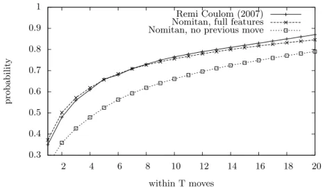
The global efficiency of the learned Bradley-Terry model can be checked on a set of games between professional players, by evaluating if the moves played by the players are in the top T moves of the Bradley-Terry model. Figure 1 shows the cumulative probability of finding the move played in the game records in the top T static P (m) values of the Bradley-Terry model. The cumulative probability with all the features of our program is close to the results of Coulom
0.3 0.4 0.5 0.6 0.7 0.8 0.9 1 2 4 6 8 10 12 14 16 18 20 probabilit y within T moves Remi Coulom (2007) Nomitan, full features Nomitan, no previous move
Fig. 1. Cumulative probability of finding the moves of the test set of game records in
the top T static values
in 2007 [3]. We have not implemented “dynamic” features like the ownership described in [3], which perhaps explain why Coulom results are better for T > 8. Also, we show the cumulative probability when the feature “distance to the previous move” of our program is disabled. We can see that the results are significantly worse. This shows that this feature is useful, despite the fact that the Markov property of the game of Go implies that the static value of a move is theoretically independent from the last move played by the opponent.
3.4 Usage of the Bradley-Terry model
It is straightforward to use the Bradley-Terry (BT) model as a policy of the Monte-Carlo simulations. For each legal move m of a given board, the BT model leads to a value P (m)∈ [0, 1], which reflects the probability that the move m would be played by a strong player. Then, a realistic simulation is obtained by selecting the move m with a probability P (m).
In this article, we focus on two other usages of the BT model, in the search tree of the UCT algorithm. We will describe first how to limit the number of searched moves, a method known as progressive widening, and then how to create an efficient static knowledge bias directly in the UCB formula.
The BT-model has also other possible applications, for example to avoid unnatural moves when playing entertaining games against human players [14].
4
Progressive widening
4.1 Progressive widening formula
Compared to other classical board games, like draughts or chess, the number of legal moves on a typical Go board in the usual 19× 19 size is very high, around
300 in the opening stage, and over 200 during most of the game. Searching all the legal moves would be unefficient, so we need to restrict the search to a small set of promising moves.
Coulom proposed the idea of progressive widening [3], which selects the top T moves with the biggest P (m) value inside the Bradley-Terry model, and widens the search when the number of playouts increases. Chaslot et al. proposed inde-pendently the idea of progressive unpruning [4], which is essentially the same. This is efficient because we know from Figure 1 that the probability of finding the best move within the top T = 20 moves of the Bradley-Terry model is as high as 84%.
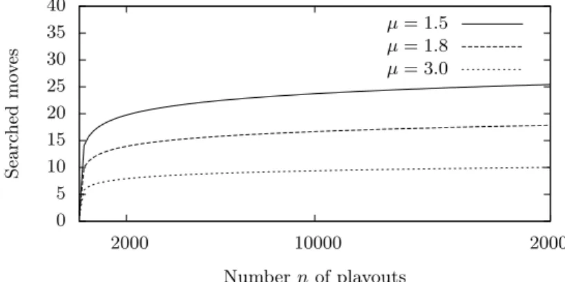
This idea is used by many programs, like Many Faces of Go [5] or Aya [13], but despite its widespread use, we have not found in the literature detailed data describing precisely the effect. We report here the results obtained with Nomitan. We use a formula close to Coulom and directly inspired by a formula of Hiroshi Yamashita, the developer of Aya [13]. With n the number of times a node has been visited, we write:
T = 1 +log n
log µ (3)
µ is a parameter that allows us to tune the formula. Figure 2 shows the num-ber of searched moves given by the formula for typical values of the µ parameter.
0 5 10 15 20 25 30 35 40 2000 10000 20000 Searc hed mo v es Number n of playouts µ = 1.5 µ = 1.8 µ = 3.0
Fig. 2. Number of searched moves in function of the number of playouts, for different
values of the µ parameter
4.2 Effect of progressing widening
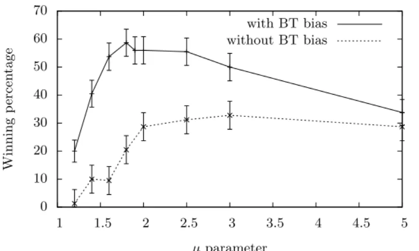
Figure 3 shows the winning rate of our program against Fuego in size 13× 13. We have done two experiments, one with the bias proposed in the next section (CBT = 0.6, K = 600), and one without. We can see that the µ parameter of progressive widening is clearly significant in both cases, and that the effect of
0 10 20 30 40 50 60 70 1 1.5 2 2.5 3 3.5 4 4.5 5 Winning p ercen tage µ parameter with BT bias without BT bias
Fig. 3. Winning rate of our program vs Fuego in function of the µ parameter
progressive widening is relatively independent of the bias proposed in the next section.
When µ is too small, the winning rate drops because the search is distributed between too many candidate moves, and so, not deep enough. On the contrary, when µ is too big, the search is focused on a too small number of candidate moves, and some important moves are not searched at all. It is interesting to note that the winning rate resists quite well to a very focused search (only 7 candidate moves are searched when µ = 5), probably because the small number of candidate moves is compensated by a deeper search that avoids local mistakes. Lastly, we can note that the best value of µ seems to be smaller when the bias of the next section is activated. This shows that it is better to search more moves, but only if the program has some way (other than only the plain UCB formula 1) to avoid the harmful scattering effect of a wider search.
5
Bradley-Terry bias in the UCB formula
We describe in this section how the Bradley-Terry model can be used as a bias in the UCB formula, and we study in detail the effect of some parameters with games against Fuego and Pachi.
5.1 Bias in the ucb formula
Adding a bias in the UCB formula is not a new idea. In fact, as far as we know, several strong Go programs like Erica [10] and Zen [6] use some kind of bias in the UCB formula to enhance the selection of some preferred moves. This need can be explained easily by the fact that, in a lot of cases, the winning ratio is almost the same between all the best candidate moves. In this kind of case, it is better to bias the choice of the move according to some policy learned offline instead of relying only on the small and noisy differences in the winning ratio.
Chaslot et al. proposed in 2009 to integrate the static knowledge with a bonus in the UCB formula [8]. They write formula 1 as follows:
µj = α· wj nj + β· prave(mj) + ( γ + C log(2 + nj) ) · Hstatic(mj) (4) where prave(mj) is the value of move mj with the RAVE heuristic, and Hstatic(mj) some static value associated to move mj according to a model learned offline. We are not sure if they also used the original exploration term of equation 1, or if it is completely replaced by the RAVE term.
The static knowledge model they used for Hstaticwas partly hand-crafted and partly learned automatically for local patterns. They report that fine-tuning of the coefficients was needed to obtain good results, a difficulty possibly coming from the conflict between the RAVE heuristic term and the static term, both terms trying to bias the search in different directions during the startup phase. In 2011, Shih-Chieh Huang proposed a related formula in his Ph.D. thesis [10]: µj= α· ( wj nj + C· √ ln n nj ) + (1− α) · prave(mj) + CP B· 1 n· Hstatic(mj) (5) Huang does not detail how Hstatic(mj) is obtained, though we guess that it is based on the Bradley-Terry model.
In both [8] and [10], the amount of experimental data showing the effect of the bias is limited. One of our goals in this article is to give more experimental evidence that such static bias is effective.
5.2 Bias based on the Bradley-Terry value
The bias that we propose here is inspired by formula 4 and formula 5. It consists of simply adding a bonus term in the UCB formula to take directly into account the value P (mj) of the Bradley-Terry model described in equation 2. In a pro-gram that already contains a Bradley-Terry model for the simulation policy or for progressive widening, this is easy and immediate to implement. Formula 1 becomes: µj = wj nj + C· √ ln n nj + CBT· √ K n + K · P (mj) (6) where CBT is the main coefficient to tune the effect (small or strong) of this bias, and K is a parameter that allows us to tune the rate at which the effect decreases. After 3K visits of the parent node, the effect is 50% of the initial value. A value of K =∞ (in practice, simply a very large value) can be used to obtain a constant bias that does not decrease with the time.
10 20 30 40 50 60 70 0 0.5 1 1.5 2 Winning p ercen tage
UCB bonus CBT coefficient
vs Pachi, K = 600 vs Fuego, K = 600 vs Pachi, K =∞ vs Fuego, K =∞
Fig. 4. Winning rate of Nomitan in function of the UCB bonus CBT coefficient
5.3 Effect of the CBT coefficient
Figure 4 shows the effect of the main CBT coefficient, against Fuego, and against Pachi, with K =∞ and K = 600. The progressive widening parameter is fixed to µ = 1.8 in this experiment.
We can see that Nomitan without the proposed bias is not so strong, with a winning rate of only 23% against Fuego and 14% against Pachi. However, with the proposed bias, Nomitan is of similar strength to these programs. With a constant bias (K = ∞), we reach 48% against Fuego and 39% against Pachi, at CBT = 0.1. The result is slightly better with a decreasing bias (K = 600), allowing us to reach 58% against Fuego and 43% against Pachi, at CBT = 0.6.
All curves display a characteristic mountain shape, which shows mainly that there is some ideal balance between the Bradley-Terry bias and the other UCB classical exploration and exploitation terms. In particular, if the bias is too big, the program will select too frequently moves with a high static value, causing some local reading mistakes.
The peak for the decreasing bias is obtained at a bigger CBT value than with a constant bias. This seems natural, since the stronger effect of the bias at the start of the search is compensated by its limited effect in the time.
5.4 Effect of the K coefficient
Figure 5 shows the effect of the K parameter, with CBT = 0.6 and CBT = 1.2. The effect of the K parameter is robust, with a large range of values where the effect is stable, for example the range [200, 2000] when CBT = 0.6.
Figure 5 also shows that for a bigger bonus, a smaller value of K is better. This simply means that a bigger bonus needs to be decreased more quickly. In fact, the two curves look essentially the same, with an horizontal shift (in logscale).
10 20 30 40 50 60 1 10 100 1000 10000 100000 Winning p ercen tage
Ucb bonus K coefficient (logscale)
CBT = 0.6
CBT = 1.2
Fig. 5. Winning rate against Fuego in function of the K parameter (logscale)
This horizontal shift can be explained with a mathematical analysis of the bias in formula 6. When the number n of playouts increases sufficiently (n≫ K), the coefficient of the bias becomes close to CBT ·
√ K·√1n.
This implies that we have somewhat similar effects for a constant value of CBT ·
√
K. In function of log K, we obtain that the curve for CBT 2 is mainly an horizontal shift of the curve for CBT 1 by 2 logCCBT 2BT 1 units. This is what we obtain on Figure 5, where the shift is 2 log1.20.6 = 0.6 units (one unit is the distance between 1 and 10, or between 10 and 100).
6
Results in size 19
× 19 and other parameters
In this section, we report results in size 19× 19 that confirm the results in size 13× 13, and we discuss the effect of some other parameters of Nomitan, which are possibly related to the efficiency of the knowledge bias.
6.1 Results in size 19× 19
In the experiments in size 19× 19, we used 5s of thinking time, which gives a number of playouts roughly similar to the 2s settings of size 13× 13 (§2.2). The number of games for each data point is around 200 games, which leads to a 95% confidence interval of±7% on the winning rate, sufficient to say that the results are significant.
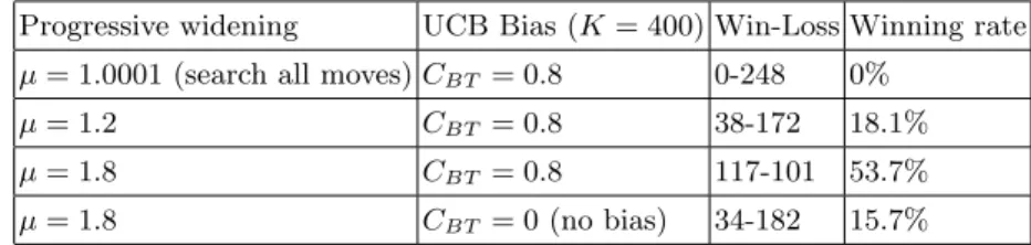
Table 1 shows the results of games against Fuego with different settings. The results are very similar to size 13× 13. The highest winning rate is obtained when both progressive widening and the knowledge bias are activated.
6.2 Final selection of the move
One of the effects of the knowledge bias in the Monte-Carlo Tree Search is an increase of the number of visits of moves with a high P (m) value. It implies that
Table 1. Winning rate against Fuego in size 19× 19
Progressive widening UCB Bias (K = 400) Win-Loss Winning rate
µ = 1.0001 (search all moves) CBT = 0.8 0-248 0%
µ = 1.2 CBT = 0.8 38-172 18.1%
µ = 1.8 CBT = 0.8 117-101 53.7%
µ = 1.8 CBT = 0 (no bias) 34-182 15.7%
the program should also rely on the number of visits of the moves, and not only on the winning ratio, when selecting the final move that will be played.
In Nomitan, the final selection is a balance between the winning ratio and the number of visits, and we have increased the weight of the number of visits after introducing the static knowledge bias.
6.3 RAVE heuristic
Contrary to most other strong Go programs, Nomitan does not use the RAVE heuristic. We have implemented a first trial, but without good results until now. It is possibly caused by the fact that many other parameters of the program have already been tuned without RAVE, making it difficult to find good parameters for RAVE.
It is not clear whether the knowledge bias described in this article would be efficient or not in a program where RAVE is already tuned and gives good results. Investigating the relationship between such bias and the RAVE heuristic is one possible direction of future research.
6.4 Features of the Bradley-Terry model
First, it must be noted that there is no need to use the same features in the Monte-Carlo simulations and in the knowledge bias. In particular, there is no need to use lightweight features in the knowledge bias.
The features chosen for the Bradley-Terry model have a direct and important effect on the efficiency of the knowledge bias. For example, against Fuego, with CBT = 0.6, K = 600 and µ = 1.8, the winning rate of our program is 29% without the “distance to the previous move” feature, and 58% when used.
This property is quite important and shows that using better and richer features in the knowledge bias is a promising direction for improving the strength of Go programs.
7
Conclusion
We have described how static knowledge about the game of Go could be learned from game records with a Bradley-Terry model, and then used in a Go program
in three different ways : to improve the Monte-Carlo simulations, to limit the number of searched moves (progressive widening), and to bias the tree search.
The first usage of the Bradley-Terry model for improving the simulations is already well-known, so we have focused on the two other usages. In particular, we have described a simple and systematic way to include the static knowledge of the Bradley-Terry model as a bonus bias in the UCB formula.
We have performed a large number of games against two open-source Go programs, Fuego and Pachi, allowing us to obtain clear experimental evidence that progressive widening and static knowledge bias are efficient. The systematic usage of the Bradley-Terry model in the three described ways allows our program to be competitive with Fuego and Pachi.
References
1. Bernd Brugmann: Monte Carlo Go. Max-Planck Institute of Physics, Tech. Rep. (1993)
2. Levente Kocsis, Csaba Szepesvari: Bandit based Monte-Carlo Planning. 17th Euro-pean conference on Machine Learning (2006) pp. 282-293
3. Remi Coulom: Computing Elo Ratings of Move Patterns in the Game of Go. Journal of the International Computer Games Association 30-4 (2007) pp. 198–208 4. G. Chaslot, M. Winands, J. Uiterwijk, H. van den Herik, B. Bouzy: Progressive
Strategies for Monte-Carlo Tree Search. New Mathematics and Natural Computa-tion 4(3), 343-357 (2008)
5. David Fotland, message on the Computer Go mailing list (2009). http://www.mail-archive.com/[email protected]/msg12628.html
6. Yoji Ojima, message on the Computer Go mailing list (2009). http://www.mail-archive.com/[email protected]/msg10969.html
7. M. Enzenberger, M. M¨uller, B. Arneson, R. Segal: Fuego - An Open-Source Frame-work for Board Games and Go Engine Based on Monte Carlo Tree Search. IEEE Transactions on Computational Intelligence and AI in Games, 2(4), 259-270. (2010) 8. G. Chaslot, C. Fiter, J.-P. Hoock, A. Rimmel, O. Teytaud: Adding expert knowledge and exploration in Monte-Carlo Tree Search. Advances in Computer Games, Lecture Notes in Computer Science Vol. 6048 (2010) pp. 1-13
9. Sylvain Gelly, David Silver: Monte-Carlo Tree Search and Rapid Action Value Es-timation in Computer Go. Artificial Intelligence, Vol. 175 Issue 11 (2011) pp. 1856-1875
10. Shih Chieh Huang: New Heuristics for Monte Carlo Tree Search applied to the Game of Go. Ph.D. Thesis, National Taiwan Normal University (2011)
11. Petr Baudis: MCTS with information sharing. Master Thesis, Charles University in Prague (2011)
12. Petr Baudis, Jean-loup Gailly: Pachi, State of the Art Open Source Go Program. Advances in Computer Games, Lecture Notes in Computer Science Vol. 7168 (2012) pp. 24-38
13. Kazuki Yoshizoe, Hiroshi Yamashita: Computer Go Theory and Practice of Monte-Carlo Method. (2012, in japanese) http://www.yss-aya.com/book2011/
14. Kokolo Ikeda, Simon Viennot: Production of Various Strategies and Position Con-trol for Monte-Carlo Go - Entertaining human players. IEEE Conference on Com-putational Intelligence in Games (2013), to be published.