資源獲得競争による昆虫の孵化および蛹化のESSタイミング

Evolutionarily

Stable

Seasonal Timing for Insects

with Competition for Renewable Resource

Hideo Ezoe

DepartmentofBiology, FacultyofScience, Kyushu University,

Fukuoka 812, Japan

資源獲得競争による昆虫の鰐化および蝋化のES $S$ タイミング

九州大学理学部生物学科 江副日出夫

I study the evolutionarily stable seasonal patterns ofhatching and pupation for herbivorousinsects that engageinexploitativecompetition for arenewable

resource.

Longer larval feeding period enhances female fecundity, but also

causes a

higher mortality by predation and parasitism. Previously, it

was

shown that the

evolutionarily stablepopulation includes asynchronous startingandendingof larval

feeding periodina model inwhich larvaJ growthrate decreases with the total larval biomass in the population due presumably to interference competition. Here I studythe

case

in which

resource

availability changes not onlywith environmental

seasonalitybut also with the depletion by the feeding oflarvae. Ifthe environment

for host plants changes fast, the ESS insect population may include synchronous timingofhatching and pupation. Ifthe impact ofthe herbivoryis strongcompared

with the speed of seasonal change ofthe environment, both hatching and pupation

should

occur

asynchronously in the ESS. In addition, ifthe environmental variable

changes as

a

symmetric function oftime, the length ofperiod in which hatching

Introduction

Insects living in temperate regions have widely diverse life histories adapted to seasonalityofthe environment. Closely related species or

even

populations ofthe same species may sometimes show greatly different life history

patterns, especially overlatitudinalgradient (Danks 1987;Kidokoro&Masaki 1978;

Masaki 1980;Furunishi&Masaki 1982;Sota 1987, 1998, 1994;Tauber et al. 1986).

Diversityin phenology, orseasonalityin life cycle, maypartially attribute to the

escape from the coldness during winter which may often require winter diapause.

Phenology is also related with seasonally changing resource availability, as well

as

coldness in winter, possibly modified by seasonalily changing risk ofpredation

and parasitism. Shapiro (1975) _{for example studied the phenology ofeight}

univoltine oak-feedinglepidopterans in the New Jerseypine barrens and observed that all the eight species have theirfeedinglarval stages in spring in spite ofgreat

differences among them in the adult season orin the overwintering stage. In this paper, I study the evolutionarily stable insect life cycle under

exploitative competition, in which the dynamics ofresource availability are

included explicitly. The resource (or _host plant) availability increases by growth

and decreases by herbivory. Bymathematical and numerical analysis I show that whether hatching and pupation

occur

synchronously depends both on the

intensityofherbivory and on the rate of seasonal change ofthe environment.

Specificallyboth pupation andhatching

occur

synchronously in the ESS

population ifthe feeding larval density is small and ifthe environnent changes

quickly, but they occur asynchronously if the impact ofherbivoryis strong

compared with seasonal change of the environment. In addition, if$bo$th hatching

and pupation occur asynchronously, the interval during which

some

pupation

occur

every day is likelyto be much longerthan a similarinterval for hatching.

Model

Consider a population ofherbivorous insects, the larvae of whichfeed on host plants with seasonal availability. Suppose that each larva in thepopulationis indexedby$i$

.

Thegrowth ratein thebodyweight $W_{i}$ ofafeedinglarva$i$ onday$t$ is,

$\frac{dW_{i}}{dt}=aR(t)W_{i}$ (1)

where $a$ is a constant for growth efficiency. Function$R(t)$ is the abundance of host

plants or resource availability. The initial size of larvae is assumed a constant $w_{0}$

which is given by the egg size.

Host plants expand their leaves and shoots for photosynthesis, which may

be damaged by feedinglarvae. Abundance of hostplants $R(t)$ changes with time

as follows:

$\frac{dR}{dt}=\{r(1-\frac{R}{K(t)})-bB\}R$ (2)

where$B(t)$ denotes total biomass of feedinglarvaein the population. Equation 2

implies that, _{when there} is no herbivory, resourcelevel $R(t)$ follows a logistic

equation with intrinsic reproductive rate $r$ and carrying capacity$K(t)$.

In themodel, a life history schedule ofa larva is specified byits hatching

date and pupationdate, i.e. the start and the end of activefeeding. To indicate the life cycle timing of

an

individual, I here introduce a feeding activity schedule instead of those two dates. The strategy of individual $i$ is represented by function

$\sigma_{i}=\sigma_{i}(t)$ such as $\sigma_{i}$ is equalto unitywhen it is fully active in feedingon day$t$,

zero when it isinactive, and takes a value between zero andunityfor an

intermediate level offeeding activity. A similar formulation

was

used for activity schedule of male frogs in the studyon the seasonal pattern of

sex

ratio (Iwasa&

Odendaal, 1984), formate searching activityformale butterflies within a day

(Iwasa&Obara, 1989), _for sex expression in discussing sex change evolution

(Iwasa, $1991b$), as_well as_forfeeding activityofbutterflylarvae(Iwasa, $1991a$).

By using $\sigma_{i}$, Equation 1 can be rewritten as the following equation, which

holds

over

the whole season$[0, T]$:

$\frac{dW_{i}}{dt}=aR(t)W_{i}\sigma_{i}$ (3a)

together with the initial condition:

$W_{i}(0)=w_{0}$ (3b)

Since $W_{i}$ does not change before hatching, $W_{i}$ on the hatching day is the same as

$w_{0}$ from Equation $3b$.

Total biomass of feeding larvae $B(t)$in the populationis the sum of weight of

all larvae multiplied bythe survivorship to day $t$ and the activityonthatday $\sigma_{i}(t)$;

$B(t)= \sum_{i}W_{i}(t)\sigma_{i}(t)\exp(-m\int_{0^{t}}\sigma_{i}(t)dt)$ (4)

Constant $m$ is the daily mortality of

an

actively feedinglarva. Note that the

sun

in

Equation 4 needs to be calculated for all the individuals includedin the initial

population with population size$N_{0}$. I here

assume

that mortality in inactive

stages is negligibly small relative to $m$.

I

assume

thatfecundity, or the expected number of eggs which

an

adult

female can lay, isproportional to its pupation size, the final body weight oflarvae

(forjustificationofthis assumption,

see

Iwasa, $1991a$; Iwasaet al., 1992, 1994). _In

particular it is equal to $W_{i}(T)$ ofthe solution ofEquation $3a$, because $W$does not

change with time afterpupation date (i.e. during $\sigma_{i}(t)=0$). The fecundityis equal

This multiplied by the larval survivorship is the fitness ofan individual adopting strategy $\sigma_{i}$:

$\phi(\sigma_{i})=Q\frac{W_{i}(T)}{w_{0}}\exp(-m\int_{0^{T}}\sigma_{i}(t)dt)$ (5)

where $\phi$ is the functional of function $\sigma_{i}$(

$\bullet$). Inthe evolutionarilystable

population, each individual chooses its own schedule offeeding activity $\sigma_{i}$ so asto

maximize its fitness $\phi(\sigma_{i})$.

Calculating derivative ofEquation 5 and using Equation $3a$, I

can

derive

$\phi(\sigma_{i})=Q\exp[\int_{0^{T}}(aR(t)-m)\sigma_{i}(t)dt]$ (6b)

When$R(t)$ is given, Equation $6b$ is maximized by choosing $\sigma_{i}(t)$

as

follows:

$aR(t)-m>0\Leftrightarrow\sigma_{i}=1$ (7a)

$aR(t)-m<0\Leftrightarrow\sigma_{i}=0$ (7化)

$aR(t)-m=0\Leftrightarrow$ $\sigma_{i}$ may have any value

between zero andone. (7c)

In the ESS population, eachindividual musthave the fitness that is no smaller than the fitness for any mutants that invade in small abundance in the

population. Hence I can conclude that all of the members in the populationmust

satisfy Equations $7a,$ $7b$, and $7c$, which indicate that all the individuals must

engage in active feeding when the resource availability $R(t)$ exceeds $m/a$, all should stay inactive when$R(t)$is less than $m/a$_, and actively feeding and inactive

individuals can coexist simultaneously only when$R(t)$ equals to $m/a$

.

Then$f_{i}$ is

the

same

between individuals for all $t$, and I

remove

the suffix $i$ of$f_{i}(t)$in the

following. It is followed thatEquation 4 and Equation $6a$

are

rewritten as

B(t)=N0f=\mbox{\boldmath $\sigma$}テ (8) and

(10)

$\phi(\sigma_{i})=Q\exp[j_{0^{T}}(aR(t)-m)\overline{\sigma}(t)dt]$ (9)

respectively. InEquation 8,$N_{0}$ denotesthe initial population of eggs atthestart of

the

season

and $\overline{\sigma}=\overline{\sigma}(t)$ is the population average of

$\sigma_{i}$, and I call it “average

activity“

on

day$t$. ThenEquation 2

can

be rewrittenas:

$\frac{dR}{dt}=\{r(1-\frac{R}{K(t)})-bN_{0}\ulcorner\sigma\}R$

Specifically I assume that a season favourable for growth of host plant lasts from the beginning $(t=0)$ to date $T_{f}(T_{f}<T)$, duringwhich carrying capacity$K(t)$

$hasasinglepeakK_{1}>m/a$

.

$AfterT_{f},$$K(t)isasmallvaluesatisfyingK_{0}<m/a$

.

Specifically I choose

$K(t)= \{K_{0}+\frac{K_{1}^{K_{0}}-K_{0}}{2}(1-\cos\frac{2\pi tt<}{T})0,$ $or_{0<t<T_{f}}t>T_{f}$ (11)

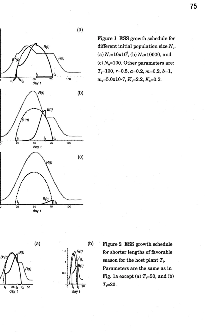
The evolutionarily stable patterns for typical cases are shownin Fig. 1 and

Fig. 2. Figure laillustrates the case in which the impactofherbivory bythe larvae

on

hostplants is large. The

season

is composed of five phases. In the beginning of

the season, both carrying capacity$K(t)$ and the resource availability$R(t)$

are

low.

Then$K(t)$ starts increasing and resource level $R(t)$ increases following$K(t)$ with

some

time delay. When$R(t)$ reaches a critical level $m/a$_, on _day $t_{1}$, some fraction

ofeggs hatches on that day. However in this particular example, some fraction of eggs remains unhatched and they hatch asynchronously over a period from $t_{1}$ to $t_{2}$

, WhichI call’hatching interval’. This is the second phase. $Ont_{2},$ $alltheeggs$

finish hatching and then engage in active feeding as larvae. This third phase of

full growth _{ends on} day$t_{3}$ , on which some fraction ofsurviving larvae enters

pupation. _{Howeverthe others remain feedinglarvae and they turn to pupae}

During this fourth phase,

resource

availability$R(t)$ remain constant $m/a$. On $t_{4}$,

all the larvae finish pupation and thereafter they experience non-feeding stages (pupa, adult, _and egg), the timing ofwhich is out ofconcern ofourpresent model.

In addition, this asynchronisation also occurs ifthe rate of change in carrying

capacity$K(t)$ is fast compared with intrinsic growth rate $r$ and growth efficiency of

larva $a$

.

In Fig. la hatching and pupation occur asynchronously. During hatching and pupation intervals, the resource availability remains constant $(R(t)=m/a)$

and the biomass ofactively feedinglarvae$B(t)$is equal to

$B^{*}(t)= \frac{r}{b}(1-\frac{m}{aK(t)})$ (12)

which canbe determined only by carrying capacity function$K(t)$. This

curve

is

illustratedin Fig. la byabroken line. On the first date ofhatchinginterval$t_{1},$$K(t)$

is greater than$R(t)=m/a$, then$B(t)$ discontinuously changes from zero to $B^{*}(t_{1})>0$.

The last date ofhatchinginterval $t_{2}$ is derived from$B^{*}(t_{2})=N_{0}w_{0}$. Note that those

individuals hatching early do not change its expected biomass during hatching

intervals, because gain bygrowth andloss by mortality cancel with each other

exactly. Similarly ifthe dayforbeginning of pupation $t_{3},$$B(t)$is greater than$B^{*}(t)$,

$B(t)$ discontinuously goes down to$B^{r}(t_{3})$. The last date ofpupationinterval $t_{4}$is

obtainedfrom$B(t_{4})=0$

.

Iftheimpact ofherbivory by thelarvae to hostplantsis not very strong,

eitherhatching or pupation or both

occur

synchronously. Figure lb is the phenology of the ESS population in which hatching occurs synchronously but

pupation

occurs

asynchronously. When $R(t)$ reaches a critical level $m/a$ on _day

$t_{1}$, the total biomass of the insectpopulation maybe smaller than the value given byEquation 12 onthat day:

$N_{0}w_{0} \leq\frac{r}{b}(1-\frac{m}{aK(t_{1})})$ (13)

Then all the eggs hatch synchronously and hatching interval does not exist. Inequality 13

can

be satisfied ifthe egg biomass ofthe insect$N_{0}w_{0}$is sufficiently

small.

This is likelyto be the case ifthe rate ofchange in seasonal carrying

capacity$K(t)$ is fast (Fig. $2b$), because$K(t)$becomesquite large onthe dayat which

resource

availability reaches the prescribed level $m/a$

.

Figure lc illustrates the case in which not only hatching but also pupation

occurs

synchronously. Whether or not the pupation occurs asynchronously in the

ESS population should also dependonthe impact of the herbivory on host plants.

During the period in which all the individuals should engage in active feeding, the

resource

availability should be larger than $m/a$

.

After the peak season, the

resource

availability starts to decline with time. The date $t_{3}$ onwhich fully active

feeding ends is determined as a date on which$R(t)$ becomes equal to $m/a$

.

Ifthe

impact of the insect feeding onthe

resource

is very $smaU,$$R(t)$is larger than$K(t)$,

as

the resource availability decreases following the decline ofcarrying capacity

$K(t)$with

some

time delay. Hence,

we

have

$K(t_{3}) \leq\frac{m}{a}$

(14)

then$B^{*}(t_{3})$isnegative. Consequently $t_{3}$is later than the date $t_{4}$ on whichEquation

14 becomes zero. This implies that all the larvae should pupate onthe same day synchronously(Fig. lc). Ifinstead the impact offeedinglarvae onthe food plant is strong,

resource

availability is smaller than the carrying capacity on day $t_{3}$, and

then there is

a

pupationinterval, asis the case forFig. la and lb. Whetherornot

pupation

_occurs

asynchronously is determined by the relative magnitude of$R(t_{3})$

and$K(t_{3})$, which in turn reflects the impact ofherbivory relative to the rate of

Discussion

Inthis paper I studied the evolutionarily stable pattern of hatching and pupation within a population ofinsects which engage in intraspecific exploitative competition for seasonally changing

resource.

I found that the hatching and

pupation timing are synchronous in the evolutionarily stable population if

seasonal environmentchanges rapidly and ifthe impact ofherbivory by the insects on host plants is small.

Previously, Iwasa (1991a) _{and Iwasa et al.} (1994) _{studied the evolutionarily}

stable seasonal timing ofhatching and pupation by theoretical models in which the larval growth rate is simply assumed as a decreasing function of the biomass offeeding larvae at that time. They concluded that the phenological timing of insects is always asynchronous. In contrast the analysis in the present paper in

which the

resource

dynamics are traced explicitly shows that both pupation and

hatching

can

be synchronous if theimpact ofherbivory tothe host plant

population is small orifthe environmental change very rapidly. It also supports

the conclusion ofthe previous works that the pupationis

more

likely to

occur

asynchronously than hatching.

A similar idea ofevolutionarily stable timing under competition for

resource

has been developed for modelling seasonality in leafexpanding activity

for terrestrialplants. Harada&Takada(1988) _{studied optimal timing of leaf}

expansion and shedding ofdeciduous trees with competition by shading in a model with twolayers ofleaves, and found that the optimal schedule is different between the two layers, which engage in asymmetric competition. Sakai (1992)

studied the evolutionarily stable timing ofleafexpansion for equivalent competitors, and found that the schedule of leafexpansion and shedding is

and shedding

can

be asynchronous under strong competition for light. This

conclusion

is qualitatively similar to the one inthis paper, although Sakai dealt with the

case

in which no reproduction or growth of

consumers

(i.e. _tree leaves)_is

considered.

In this paper, I adopted several simplifying assunptions, some ofwhich may be removedin the future theoretical works. First, I assumedthatdaily

growthrate is proportional to the larval bodyweight in Equation 1 and that the number of eggs female can layis also proportional to its pupation weight in

Equation 4. However it is more plausible that female fecundity increases with her

body weightbut saturates for averylarge body weight. Second, the growthrate is

assumed

to be proportionalto the resource availabilityin Equation 1. In realityit

is

more

likely that the growth rate would saturate for verylarge

resource

availability, and also that the saturationlevel would increase with the larval body

weight because larger larva is

more

mobile andis able to sequester more

resource.

This effect

was

consideredin Iwasaet al. $(1992, 1994)$ in a model without resource

dynamics. Third, the competitors may be sibs or half-sibs from the same clutch

laidby a single mother. Then we need the analysisincluding kin selection. These modifications would be important future theoretical study ofinsect life cycle from the viewpoint ofevolutionaryecology.

References

Danks, H.V. (1987) _Insect dormancy: an ecological perspective. Biological Survey

ofCanada, Ottawa. 439pp.

Furunishi, S. &Masaki, S. (1982) _{Seasonallife cycle intwo species of ant-lion} (Neuro _tera: Mvrmeleontidae). $Jpn$. J. Ecol. 32, 7-13.

Harada, Y. &Takada, T. (1989) Optimal timingof leafexpansion and sheddingin

Iwasa, Y. and Y. Obara, (1989) _Agame model for the daily activity schedule of the malebutterfly. J. Insect Behav. 2, 589-608.

Iwasa, Y. (1991a) _{Asynchronous pupation ofunivoltine} insects as the

evolutionarilystablephenology. Res. Poupl. Ecol. 33, _213-27.

Iwasa, Y. (1991b) Sex change evolution and cost ofreproduction.Behav. $Eco$

.

$2,56-$

ae.

Iwasa, Y., Ezoe, H. &Yamauchi, A. (1994) _{Evolutionarily stable seasonal timing of}

univoltine and bivoltine insects. InInsect life-cycle polymorphism: theory,

evolution and ecological consequences

_for

seasonality and diapause

control. (H.V. _{Danks and S.} Masaki, eds.) _{Kluwer Academic}Publ, MA, USA

(in press).

Iwasa, Y. &Odendaal, F.J. (1984) _{A theoryon the temporal pattern ofoperational}

sex ratio: The active-inactive model.Ecology 65, _886-93.

Iwasa, Y., Yamauchi, A. &Nozoe, S. (1992) Optimal seasonal timing ofunivoltine

and bivoltine insects.Ecol. Res. 7, 55-62.

Kidokoro, T. &Masaki, S. (1978) _{Photoperiodic responsein relationto variable}

voltinism in the ground cricket, Pteronemobius $fasci_{-}Des$ Walker

(Orthoptera: Gryllidae).$Jpn$

.

J. Ecol. 28, 291-8.

Masaki, S. (1980) _{Summer diapause.A. Rev.} $Ent$

.

_{$25,1- 25$}

.

Sakai, S. (1992) _{Asynchronous leafexpansion and shedding in} a _seasonal

environment: result ofa competitive game. J. theor.Biol. 154, 77-90.

Shapiro, A.M. (1975) _{The temporal} components ofbutterfly species diversity. In: Ecology and Evolution ofCommunities. (M.L. Cody&J.M. Diamond, eds.),

Belknap, HarvardUniv., Cambridge, MA. pp. 181-95.

Sota, T. (1987) Mortalitypattern and age structure in two carabid populations with different seasonal life cycles. Res. Popul. Ecol. 29, 237-54.

Sota, T. (1988) _{Univoltine and bivoltine life cycles ininsects:}

a

_{model with}

density-dependent selection. Res. Popul. Ecol. 30, _134-44.

Sota, T. (1994) _{Variation of carabidlife cycles alongclimatic gradients: an}

adaptive perspective for life history evolution under adverse conditions. In

Insect life-cycle polymorphism: theory, evolution and ecological

consequences

_for

seasonality and diapause control. (H.V. _{Danks and S.}

Masaki, eds.), _{Kluwer Academic} Publ, MA, USA (in press).

Tauber, M.J., Tauber, C.A.

&Masaki,

S. (1986) _{Seasonal adaptations}

_of

_insects.

Figure 1 ESSgrowth schedulefor

differentinitial populationsize$N_{0}$.

(a)$N_{0}=10x10^{6},$_{$(b)N_{0}=10000$}, and

(c)$N_{0}=100$. Otherparameters are: $T\ulcorner-100,$$r=0.5,$ $a=0.2,$ $m=0.2,$$b=1$, $w_{0}=5.0x10- 7,$ $K_{1}=2.2,$ $K_{0}=0.2$.

(b) Figure2 ESS growth schedule

forshorterlengths of favorable

seasonfor thehostplant$T_{f}$

.

Parametersarethesame asin

Fig. la except(a) $T_{\overline{\ulcorner}}50$,and(b) $T\ulcorner-20$

.