Local Moves Generating Writhe Polynomials of Virtual Knots (Intelligence of Low-dimensional Topology)

全文

(1)107. Local Moves Generating Writhe Polynomials of Virtual Knots. Takuji Nakamura (Osaka Electro‐Communication University) Yasutaka Nakanishi (Kobe University) Shin Satoh (Kobe University) 1. Introduction. This paper is a résumé of the paper [8]. The odd writhe J(K) is one of fundamental invariants of a virtual knot K (cf. [5]). In [10], Taniguchi and the third author intro‐ duced local moves called :‐moves and proved that :‐moves correspond to the odd writhe; namely, two virtual knots have the same odd writhe if and only if they are related by a finite sequence of 三‐moves. On the other hand, there is another invariant of a virtual knot K called the writhe. polynomial W_{K}(t) (cf. [1, 6, 10]). The writhe polynomial is stronger than the odd writhe in the sense that J(K)=-W_{K}(-1)/2 holds. Therefore, it is natural to ask which local moves correspond to the writhe polynomial.. In Section 2, we introduce local moves for virtual knots and links called shell moves. In Section 3, we prove that the writhe polynomial correspond to shell moves. In Section 4, we study which invariants of a 2‐component virtual link correspond to shell moves.. 2. Gauss diagrams. A Gauss diagram consists of a finite number of oriented circles and oriented, signed chords equipped with signs of endpoints as shown in Figure 1. \prime.<'\cdots\cdot. \prime^{\prime'}. \prec\cdots\cdot. \prime\prec-\ dot\cdot\cdot\cdot\backsla h\backsla h\backsla h. \dot{j}. Figure 1: Self‐ and nonself‐chords of a Gauss diagram. A \mu ‐component virtual link is an equivalence class of Gauss diagrams with. \mu. circles up. to Reidemeister moves RI‐R3 (cf. [4, 5]). See Figure 2. If \mu=1 , it is called a virtual knot.. The first author is partially supported by JSPS Grants‐in‐Aid for Scientific Research (C), 17K05265 . The second author is partially supported by JSPS Grants‐in‐Aid for Scientific Research (C), 19K03492 . The third author is partially supported by JSPS Grants‐in‐Aid for Scientific Research (C), 19K03466..

(2) 108. R2. R2. \sim. \sim. \sim R3. Figure 2: Reidemeister moves for Gauss diagrams. The shells for a chord \gamma are parallel self‐chords which are oriented with respect to the sign of the endpoint of \gamma as shown in Figure 3. We remark that a shell in this paper is a. special case of an anklet in [7].. Figure 3: Shells for. \gamma. The shell moves Sl and S2 are local moves defined by using Gauss diagrams as shown in Figure 4. Precisely, an Sl‐move slides a shell along a chord to the opposite side with the same sign, and an S2‐move changes the position of the adjacent endpoints of chords with making a pair of shells with respect to the signs of the endpoints. S1. \sim. Figure 4: Shell moves Sl and S2. We say that two Gauss diagram are S‐equivalent if they are related by a finite sequence of Reidemeister moves and shell moves, and two virtual links are S‐equivalent if their Gauss diagrams are S ‐equivalent..

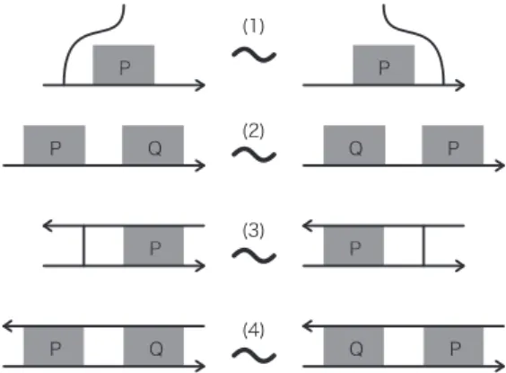
(3) 109 Lemma 2.1. If two Gauss diagrams are related by a deformation (1) or (2) as shown in Figure 5, then they are S‐equivalent. the su. of. signs. y. \square. (1) \sim. \sim_{-\delta_{1}^{-} (2) Figure 5:. S ‐equivalent. \Sigma^{\delta_{J}\delta_{j}. Gauss diagrams in Lemma 2.1. Lemma 2.2. If two Gauss diagrams are related by a deformation (1) -(4) as shown in Figure 6, then they are S‐equivalent. Here,. P. and Q are portions of whole chords.. \square. (1) \sim. \sim(2) (3) '. (4) \sim. Figure 6:. S ‐equivalent. Gauss diagrams in Lemma 2.2. Let G be a Gauss diagram with \mu circles C_{1} , . C_{\mu} . For n\in \mathbb{Z} and 1\leq i\neq j\leq\mu, we define the n ‐snail of type i and the n ‐snail of type (i, j) to be the portion of chords as shown in Figure 7. Then we have the following.. Lemma 2.3. If two Gauss diagrams are related by a deformation (1) -(4) as shown in Figure 8, then they are S‐equivalent.. \square. By using Lemmas 2.1−2.3, we have the following standard form of a Gauss diagram up to S ‐moves..

(4) 110. um. 0\dagger. =-\epsilon n. \in S_{i}(n) \epsilon 5_{ij}(n). Figure 7: The (1) \sim. n. ‐snails \varepsilon S_{\dot{i} (n) and \varepsilon S_{ij}(n) (2) \sim. c_{i}arrow (3). C_{j}arrow. \sim. C_{i}arrow (4) \sim. \subset_{i}arrow. Figure 8:. S ‐equivalent. Gauss diagrams in Lemma 2.3. Proposition 2.4. Any Gauss diagram of an oriented \mu ‐component virtual link is S‐ equivalent to a Gauss diagram G with \mu circles C_{1} , . C_{\mu} which satisfies the following conditions. Figure 9 shows the case \mu=3.. (i) The chords of. G. (ii) There is an arc. form a finite number of snails. \alpha_{i}. on each C_{i} such that all snails of type. i. spans. \alpha_{i}.. (iii) All snails of type (i, j) spans (C_{i}\backslash \alpha_{i})\cup(C_{j}\backslash \alpha_{j}) in parallel. (iv) There is no snails \pm S_{i}(0) or\pm S_{i}(1) for any. i.. (v) There is no pair of snails +S_{i}(n) and-S_{\dot{i}}(n) for any. i. and. n.. (vi) There is no pair of snails +S_{\dot{\iota}j}(n) and-S_{ij}(n) for any i\neq j and. 3. The case. \mu=1. In this section, we consider an oriented virtual knot circle. C.. For portions P_{1} , .. K. and its Gauss diagram. P_{k} of chords, we denote by. as shown in Figure 10. For integers copies of \varepsilon S(n) , where \varepsilon is the sign of. Lemma 3.1. Any Gauss daigram of a_{n}\in \mathbb{Z}.. \square. n.. a,. ( \sum_{i=1}^{k}P_{i}). G. with a. the Gauss diagram. n\in \mathbb{Z}, aS(n) denotes the concatenation of |a|. a.. K. is. S ‐equivalent. to. ( \sum_{n\neq 0,1}a_{n}S(n). for some \square.

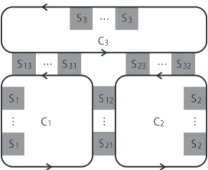
(5) 111 111. Figure 9: A Gauss diagram with three circles. Figure 10: The Gauss diagram. A chord \gamma divides the circle C into two arcs. Let. \alpha. ( \sum_{i=1}^{k}P_{i}) be the one oriented from the initial. to the terminal endpoint of \gamma . We define the index of \gamma to be the sum of signs of endpoints of chords on \alpha . For each n\neq 0 , the sum of signs of all chords whose index is equal to n defines an invariant of K . It is called the n ‐writhe of K and denoted by J_{n}(K) . The writhe polynomial is defined by. W_{K}(t)= \sum_{n\neq 0}J_{n}(K)(t^{n}-1)\in \mathbb{Z}[t, t^{-1}]. Refer to [1, 2, 6, 10] for more details. Lemma 3.2. Let K be an oriented virtual knot.. (i) The writhe polynomial W_{K}(t) is invariant under S‐moves. (ii) If. K. is presented by a Gauss diagram given in Lemma 3.1, then we have. W_{K}(t)= \sum_{n\neq 0,1}a_{n}t^{n}-(\sum_{n\neq 0,1}na_{n})t+\sum_{n\neq 0,1} (n-1)a_{n}. \square. By Lemma 3.1 and Lemma 3.2(ii), we have the following. Proposition 3.3. Let K and K' be oriented virtual knots. If W_{K}(t)=W_{K'}(t) holds, \square then K and K' are S‐equivalent..

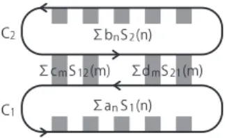
(6) 112 Therefore the following holds by Lemma 3.2(i) and Proposition 3.3. and K' , the following are equivalent.. K. Theorem 3.4. For two oriented virtual knots. (i) W_{K}(t)=W_{K'}(t) . (ii) 4. K. and. K'. are related by a finite sequence of shell moves.. The case. \square. \mu=2. In this section, we consider an oriented 2‐component virtual link L=K_{1}\cup K_{2} and its Gauss diagram G with a pair of circles C_{1} and C_{2} . By Proposition 2.4, we have the following.. Lemma 4.1. Any Gauss daigram of. L. is. S ‐equivalent. to a Gauss diagram. ( \sum_{n\neq 0,1}a_{n}S_{1}(n), \sum_{n\neq 0,1}b_{n}S_{2}(n);\sum_{m\in Z} c_{m}S_{12}(m), \sum_{m\in Z}d_{m}S_{21}(m) a_{n}, b_{n}(n\neq 0,1) and c_{m}, d_{m}(m\in \mathbb{Z}) as shown in Figure 11. Here, the entries present the concatenations of snails of type 1, 2, (1, 2), and (2, 1), respectively. \square. for some integers. Figure 11: A Gauss diagram of an oriented 2‐component virtual link. For (i, j)=(1,2) or (2, 1), the (i, j) ‐linking number of. L,. denoted by Lk(K_{i}, K_{j}) , is. defined to be the sum of signs of all nonself‐chords oriented from C_{i} to C_{j} . The virtual. linking number of L is defined by \lambda(L)=Lk(K_{1}, K_{2})-Lk(K_{2}, K_{1}) [9] (cf. [3]). It is easy to see that Lk(K_{1}, K_{2}), Lk(K_{2}, K_{1}) , and \lambda(L) are invariant under S ‐moves. If \lambda(L)<0 , then by switching the roles of K_{1} and K_{2} , the case reduces to \lambda(L)>0. In what follows, we may assume that \lambda(L)\geq 0 . We denote \lambda(L) by \lambda for simplicity. The following propositions give standard forms of. L. up to S ‐equivalence.. Proposition 4.2. Let G be a Gauss diagram of. L.. (i) If \lambda\geq 1 , then. G \sim(\sum_{n\neq 0,1-\lambda,-\lambda+1}a_{n}S_{1}(n),\sum_{n\neq 0,1 \lambda,\lambda+1}b_{n}S_{2}(n). ;.

(7) 113. \sum_{m=0}^{\lambda-1}c_{m}S_{12}(p+m),\sum_{m=0}^{\lambda-1}d_{m}S_{21}(-p-m) ). for some integers a_{n}(n\neq 0,1, -\lambda, -\lambda+1), b_{n}(n\neq 0,1, \lambda, \lambda+1), \lambda-1) , and p.. (ii) In particular, if. \lambda=1 ,. c_{m},. d_{m}(0\leq m\leq. then. G \sim(\sum_{n\neq 0,1,-1}a_{n}S_{1}(n), \sum_{n\neq 0,12},b_{n}S_{2}(n);c_{0} S_{12}(0), d_{0}S_{21}(0) for some integers a_{n}(n\neq 0,1, -1), b_{n}(n\neq 0,1,2),. c_{0} ,. and d_{0}.. \square. Proposition 4.3. We have the following S‐equivalent Gauss diagrams.. (i) If. \lambda=0 ,. then. (P, Q; \sum_{m\in \mathb {Z} c_{m}S_{12}(m),\sum_{m\in \mathb {Z} d_{m}S_{21} (m) \sim(P, Q;\sum_{m\in \mathb {Z} c_{m}S_{12}(m+k),\sum_{m\in \mathb {Z} d_{m}S_ {21}(m-k). for any k\in \mathbb{Z}.. (ii) If \lambda\geq 2 , then. (P, Q; \sum_{m=0}^{\lambda-1}c_{m}S_{12}(p+m),\sum_{m=0}^{\lambda-1}d_{m}S_{21} (-p-m) \sim(P, Q;\sum_{m=0}^{\lambda-1}c_{m}'S_{12}(p'+m),\sum_{m=0}^{\lambda-1}d_{m} 'S_{21}(-p'-m). ,. where. \{ begin{ar ay}{l} (c\'{O},. c_{\lambda-k1}',c_{\lambda-k}',\ldots,c_{\lambda-1}')=(c_{k}, \ldots,c_{\lambda-1},c_{0},\ldots,c_{k-1}), (d\'{O} d_{\lambda-k1}',d_{\lambda-k}',\ldots,d_{\lambda-1}')=(d_{k}, \ldots,d_{\lambda-1},d_{0},\ldots,d_{k-1}), \end{ar ay} and. p'=p+k- \sum_{i=0}^{k-1}(c_{i}-d_{i}). for any. k. with 1\leq k\leq\lambda-1.. \square. A self‐chord \gamma spanning C_{i} divides C_{i} into two arcs. Let \alpha be the one oriented from the initial to the terminal endpoint of \gamma in C_{i} . we define the index of \gamma in G to be the sum of signs of endpoints of self‐ and nonself‐chords on \alpha . For n\in \mathbb{Z} and i=1,2 , the sum of signs of all self‐chords whose indices are equal to n defines the invariants J_{n}(K_{1};L) for n\neq 0, -\lambda and J_{n}(K_{2};L) for n\neq 0, \lambda . These are called the n ‐writhes of K_{1} and K_{2} in L, respectively..

(8) 114 On the other hand, for nonself‐chords \gamma and \gamma_{0} , the relative index of \gamma with respect to to be the index of \gamma in the Gauss diagram obtained from G by surgery along \gamma_{0} . For n\in \mathbb{Z} and (i, j)=(1,2), (2,1) , let J_{n}^{ij}(G;\gamma_{0}) denote the sum of signs of nonself‐chords \gamma oriented from C_{i} to C_{j} whose relative index with respect to \gamma_{0} are equal to n . Put \gamma_{0}. F_{ij}(t; \gamma_{0})=\sum_{n\in \mathb {Z} J_{n}^{ij}(G;\gamma_{0})t^{n}. For an integer s\geq 0 , let \Lambda_{s} denote the Laurent polynomial ring \mathbb{Z}[t, t^{-1}]/(t^{s}-1) . In particular, we have \Lambda_{0}=\mathbb{Z}[t, t^{-1}] and \Lambda_{1}=\mathbb{Z} . We consider an equivalence relation on \Lambda_{s}\cross\Lambda_{s} such that (f_{1}(t), g_{1}(t)) and (f_{2}(t), g_{2}(t)) are equivalent if there is an integer k with. f_{2}(t)=t^{k}f_{1}(t). and. g_{2}(t)=t^{-k}g_{1}(t) .. We denote by [f(t), g(t)] the equivalence class represented by (f(t), g(t)) , and by \Gamma(s) the set of such equivalence classes. Then the equivalence class [F_{12}(t;\gamma_{0}), F_{21}(t;\gamma_{0})]\in\Gamma(\lambda) defines the invariant of L. (cf. [2]). We call it the linking class of L and denote it by F(L) . In particular, F(L)= (Lk(K_{1}, K_{2}), Lk(K_{2}, K_{1}))\in \mathbb{Z}\cross \mathbb{Z} for \lambda=1 . Then by Propositions 4.2 and 4.3, we have. the following. Theorem 4.4. Let L=K_{1}\cup K_{2} and L'=K_{1}'\cup K_{2}' be oriented 2‐component virtual links with \lambda=\lambda'=0 . Then L and L' are related by a finite sequence of shell moves if and only if. (i) J_{n}(K_{1};L)=J_{n}(K_{1}';L') for any n\neq 0,1, (ii) J_{n}(K_{2};L)=J_{n}(K_{2}'; L') for any n\neq 0,1 , and (iii) F(L)=F(L') . \square. Theorem 4.5. Let L=K_{1}\cup K_{2} and L'=K_{1}'\cup K_{2}' be oriented 2‐component virtual links with \lambda=\lambda'=1 . Then L and L' are related by a finite sequence of shell moves if and only if. (i) J_{n}(K_{1};L)=J_{n}(K_{1}';L') for any n\neq 0,1, -1, (ii) J_{n}(K_{2};L)=J_{n}(K_{2}'; L') for any n\neq 0,1,2 , and. (iii) F(L)=F(L') . \square. Theorem 4.6. Let L=K_{1}\cup K_{2} and L'=K_{1}'\cup K_{2}' be oriented 2‐component virtual links with \lambda=\lambda'\geq 2 . Then L and L' are related by a finite sequence of shell moves if and only if.

(9) 115 (i) J_{n}(K_{1};L)=J_{n}(K_{1}';L') for any n\neq 0,1, -\lambda, -\lambda+1, (ii) J_{n}(K_{2};L)=J_{n}(K_{2}'; L') for any n\neq 0,1, \lambda, \lambda+1, (iii) F(L)=F(L') , and. (iv) J_{1}(K_{1};L)+J_{-\lambda+1}(K_{1};L)+J_{1}(K_{2};L)+J_{\lambda+1}(K_{2};L) =J_{1} (Kí; L' ) +J_{-\lambda+1} (Kí;. L' ). +J_{1}(K_{2}';L')+J_{\lambda+1}(K_{2}';L') . \square. References. [1] Z. Cheng, A polynomial invariant of virtual knots, Proc. Amer. Math. Soc. 142 (2014), no. 2, 713‐725. [2] Z. Cheng and H. Gao, A polynomial invariant of virtual links, J. Knot Theory Ram‐ ifications 22 (2013), no. 12, 1341002, 33 pp. [3] L. C. Folwaczny and L. H. Kauffman, A linking number definition of the affine in‐ dex polynomial and applications, J. Knot Theory Ramifications 22 (2013), no. 12, 1341004, 30 pp.. [4] M. Goussarov, M. Polyak, and O. Viro, Finite‐type invariants of classical and virtual knots, Topology 39 (2000), no. 5, 1045‐1068.. [5] L. H. Kauffman, Virtual knot theory, European J. Combin. 20 (1999), no. 7, 663‐690. [6] L. H. Kauffman, An affine index polynomial invariant of virtual knots, J. Knot Theory Ramifications 22 (2013), no. 4, 1340007, 30 pp. [7] T. Nakamura, Y. Nakanishi, and S. Satoh, A note on coverings of virtual knots, available at arXiv: 1811. 10852. [8] T. Nakamura, Y. Nakanishi, and S. Satoh, Writhe polynomials and shell moves for virtual knots and links, in submission.. [9] T. Okabayashi, Forbidden moves for virtual links, Kobe J. Math. 22 (2005), no. 1‐2, 49‐63.. [10] S. Satoh and K. Taniguchi, The writhes of a virtual knot, Fund. Math. 225 (2014), no. 1, 327‐342.. Department of Engineering Science Osaka Electro‐Communication University Osaka 572‐8530. JAPAN. E‐mail address:. n. ‐[email protected].

(10) 116 Department of Mathematics Kobe University Kobe 657‐8501. JAPAN. E‐mail address: [email protected]‐u.ac.jp, [email protected]‐u.ac.jp.

(11)