A NOTE ON AN OVERDETERMINED PROBLEM WITH NON-CONSTANT NEUMANN BOUNDARY CONDITION (Geometry of solutions of partial differential equations)

A NOTE ON AN OVERDETERMINED PROBLEM WITH

NON-CONSTANT NEUMANN BOUNDARY CONDITION

CHIARABIANCHINI, PAOLO SALANI

ABSTRACT. Wereview someresultsabout avariant of the Saint-Venant problem and

about a related overdetermined problem. The latter is a generalization of the Serrin

problem where the overdetermination reads $\nabla u(x)=g(x)$ on the boundary of the

unknowndomain,and$g$:$\mathbb{R}^{N}arrow[0, \infty)$ isagivenfunction. Weanalyzesomegeometric

properties ofthe solution $\Omega$ in relation with

$g$ and weprove some new results about

the continuity of$\Omega$ with respect

to $g$, assuming$g$ is an homogeneousfunction.

1. INTRODUCTION

An overdetermined problem usually consists in a Dirichlet problem given in an un-known domain, _{whose solution satisfies some extra condition (classically a Neumann}

boundary condition) which determines univocally the shape ofthe domain itself. Then

the solution of the problem is given by a couple domain-function, where the former is

the real object of research. The most famous overdetermined problem is probably the

following:

(1) $\{\begin{array}{ll}-\triangle u=1 in \Omega,u=0 on \partial\Omega,|\nabla u|=c on \partial\Omega,\end{array}$

where $c>0$ is a given constant. In a famous paper Serrin [28] proved that, under

suitable regularity assumptions, if a solution to this problem exists, then $\Omega$ must be a

ball $B(O, R)$ _and $u(x)=(R^{2}-|x|^{2})/(2n)$. After _{Serrin, a large amount of literature}

has beenproduced about variants of (1), often dealing with similar problems where the

Laplacian is substituted bysomeother operator $and,Jhe$ overdetermination writes again

as $u=0$ and $|\nabla u|=$ constant on $\partial\Omega$; but also other kinds of

overdetermined conditions have been considered in hterature, see for instance [4, 6, 14, 15, 17, 20, 27, 29, 30] and references therein. Moreover, related stability issues have been investigated, see for

instance [3, 8, 16].

Here we consider the following generalization of (1): given a function $g$ : $\mathbb{R}^{N}arrow$

$[0, +\infty)$, positive outside the origin, we investigate the problem

More precisely: for any bounded open set $\Omega$, we denote by

$u\Omega$ the stress

function

of $\Omega,$

that is the solution ofthe torsion problem:

(3) $\{\begin{array}{ll}-\triangle u\Omega=1 in \Omega u\Omega=0 on \partial\Omega,\end{array}$

or its weakform

(4) $u\Omega\in H_{0}^{1}(\Omega)$ : $\int_{\Omega}\nabla u\Omega\nabla v=\int_{\Omega}u\Omega v$ $\forall v\in H_{0}^{1}(\Omega)$

.

Then we askwhether a domain $\Omega$ exists such that the solution of (3) satisfies

(5) $|\nabla u\Omega(x)|=g(x) x\in\partial\Omega,$

and we investigate some geometric properties of$\Omega$ in connection with the properties of

the assigned function $g.$

Letusquotethatthe

same

overdeterminedconditions (5) have been alreadyconsidered

for differential problems of the torsion and of the Bernoulli types in [1, 2, 5, 19, 22].

Theoverdetermined problem (2) is naturally linked totheshape optimization problem we describe here below. Let $J$ be the functional defined

as

theopposite of the torsional

rigidity:

(6) $J( \Omega)=\frac{1}{2}\int_{\Omega}|\nabla u_{\Omega}|^{2}dx-\int_{\Omega}u\Omega dx=-\frac{1}{2}\int_{\Omega}u\Omega dx=-\frac{1}{2}\int_{\Omega}|\nabla u\Omega|^{2}dx.$

and let

(7) $\phi(\Omega):=\int_{\Omega}g^{2}(x)dx.$

The shape optimization problem consistsin minimizing $J$ with the constraint $\phi(\Omega)\leq 1,$

i.e.

(8) lnin$\{J(\Omega):\phi(\Omega)\leq 1\}.$

Notice that (8) is a variant of the famous Saint-Venant problem. This consists in

looking for the domainwith given areawhich has maximal torsionalrigidity; the answer

is the ball,

as

proved by G. Poly\‘a [25]. Here we consider the same problemin the class

of non-uniformly dense sets, whose density is driven by the function$g.$

We also recall that problem (8) is close to the one considered by B. Gustafsson and

H. Shahgholian in [19]. Indeed they study the partial differential equation $-\triangle u=f,$

where $f$ is a function (or a measure) whose positive part $(f)^{+}= \max\{0, f\}$ has compact

support, which is not our case.

In [7], the authors proved that problem (11) admits a solution (in the class of quasi-open sets) under the assumptions

(9) $g(x)>0$ for $x\neq 0,$ $\lim$ _{$g(x)=+\infty.$} $|x|arrow+\infty$

On the other hand, the simple existence of a solution to the shape optimization

problem (8) does notguaranteetheexistenceofa solutionof theoverdeterminedproblem

(2). To encounter this problem, in [7] the following assumption on $g$ is considered:

(10) $\{\begin{array}{l}g :\mathbb{R}^{N}arrow \mathbb{R} positively homogeneous of degree \alpha(i.e.g(tx)=t^{\alpha}g(x)\forall t>0, \forall x\in \mathbb{R}^{N}) ,g H\"{o} lder continuous, g>0 outside 0.\end{array}$

Thanks to (10), it is possible to find a solution $\Omega$ to problem (2) and to prove a series

ofproperties ofsuch asolution.

In Section 2 we recallsome basic properties and results about the shape optimization problem _{(8) and its connection with the overdetermined problem (2). In Section 3 we}

review some basic properties of the solution of (2) and its geometric properties, like

starshape, convexity, Steiner symmetry. In Section 4 we give

some

new results about the continuity of $\Omega$ with respect to

9. Notice that most of the results recalled in this

paper are taken from [7]. Precisely only Lemma 4.2, Corollary 4.3) and Theorem 4.4

contain original results, while Theorem 3.2 is aslight improvement of the corresponding

result of [7].

2. THE SHAPE OPTIMIZATION PROBLEM

Letus consider theenergy functional$J$defined in (6). It is easilyseenby the maximum

principle that $J$ is decreasing with respect to set inclusion, that is

$J(\Omega_{1})\geq J(\Omega_{2})$ if $\Omega_{1}\subset\Omega_{2}.$

Problem (8) consists in minimizing $J(\Omega)$ among open sets satisfying

(11) $\phi(\Omega)=\int_{\Omega}g^{2}dx\leq 1.$

Notice that the

measure

ofa set $\Omega$ satisfying (11) must be bounded

if$g(x)arrow+\infty$ as

$|x|arrow\infty$

.

Thanks to this, it is possible to prove the following.

Theorem 2.1. Underassumption (9), there exists a quasi-open set $\Omega$ solving the shape

optimizationproblem (8).

The proof in [7] follows the lines of [18] (see also [21]) and uses a

concentration-compactness argument as in [11] to prove the existence of a minimizer which is

quasi-open and may be unbounded. We refer to [21] for a precise definition and discussion of

the concept of quasi-open sets; here wejust say that, roughly speaking, quay-open sets

are super level sets offunctions in $H^{1}(\mathbb{R}^{N})$.

Apart from theproofof existence, in the restof the paper [7] thefunction$g$is assumed

to be homogeneous, precisely tosatisfy assumption (10). This makes problem (8) easier

and with a nice behavior with respect to homotheties. More precisely, for every $t>0,$

$\Omega\subset \mathbb{R}^{N}$, it holds

$J(t \Omega) = -\frac{1}{2}\int_{t\Omega}t^{2}u_{\Omega}(x/t)dx=t^{2+N}J(\Omega)$,

where the first equality follows from the fact that the stress function of$t\Omega$ is

(12) $u_{t\Omega}(x)=t^{2}u\Omega(x/t)$

.

Then using the notion of local shape subsolution introduced in [12], it is proved that the minimizer is in fact bounded and it is possible to obtain its regularity as in [9]

(see also [10]). The main difficulty is to prove that the solution $\Omega$ is actually an open

set. Once proved this, one can get higher regularity by classical techmiques from free

boundary problems like in [5] and [19].

Theorem 2.2. Under assumption (10) the shape optimization problem (8) admits a

solution$\Omega$.

If

$\alpha\neq 1,$ $\Omega$ is connected. Moreover, in dimension$N=2$ the solutionis $C^{1,\beta}$

for

some

$\beta>0$; in dimension $N\geq 3$, the reduced boundary $\partial_{red}\Omega$ is $C^{1,\beta}$ and$\partial\Omega\backslash \partial_{red}\Omega$

has

zero

$(N-1)$

_-Hausdorff

measure$\cdot.$

Thanks

to (12) the existence of

a

solution to the overdetermined problem (2) follows

by choosing a suitable dilation of

a

solution of (8).

Corollary 2.3. Let $g$ satisfy (10)

for

some $\alpha>0,$ $\alpha\neq 1$. Then there exists a solution

to the overdetemined Free Boundary Problem (2).

Remark 2.4. Notice that the case $\alpha=1$ is special, as it can be seen by considering the

mdially symmetric situation, where it is possible to have either no solution oran

_infinite

number

_of

solutions.

3. THE OVERDETERMINED PROBLEM AND THE GEOMETRY OF $\Omega$ Under assumption (10) with

$\alpha>1$

several geometric properties of the solutions of the overdetermined problem (2) are

proved in [7]. The first one is the fact that the origin $O$ must be inside the domain.

This property may look rather technical, but it is fundamental to obtain many other

properties ofthe solution.

Proposition 3.1. Assume that $g$

satisfied

(10) with $\alpha>1$

.

Let $\Omega$ be a solution

of

the

minimization problem (8). Then the $ori$gin $O$ is inside $\Omega.$

Then the monotonicity of $\Omega$ with respect to

$g$ is proved. Here we present a shght

improvement ofthe corresponding result in [7].

Theorem 3.2. Let $\Omega_{1},$$\Omega_{2}$ be (regular enough) bounded solutions to Problem (2) related

to$g_{1}$ and92, respectively, with $O\in\Omega_{i}$

for

$i=1,2$

.

Assume that

for

some $\alpha>1$ at least

one between the following two assumptions hold.$\cdot$

(13) $g_{1}(tx)\geq t^{\alpha}g_{1}(x)$

for

$t>0,$ $x\in \mathbb{R}^{N},$ $or$

(14) $g_{2}(tx)\leq t^{\alpha}g_{2}(x)$

for

$t>0,$ $x\in \mathbb{R}^{N},$

Proof.

The proof is very similar to the proof of [7, Theorem 3.2], but we give it for completeness.

Assume that (13) holds and

assume

by contradiction $\Omega_{1}\not\subset\Omega_{2}$. Then

$t= \sup\{s>0:s\Omega_{1}\subseteq\Omega_{2}\}<1.$

Furthermore $t>0$ for $O\in\Omega_{2}$ and $\Omega_{1}$ is bounded.

Consider the set $t\Omega_{1}:t\Omega_{1}\subseteq\Omega_{2}$; there exists $\overline{x}\in\partial(t\Omega_{1})\cap\partial\Omega_{2}$, with $\nu_{t\Omega_{1}}(\overline{x})=$

$\nu\Omega_{2}(\overline{x})=\nu$, where $\nu_{\Omega}(x)$ denotes the outer unit normal to $\partial\Omega$ at

$x.$

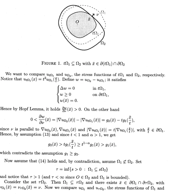
FIGURE 1. $t\Omega_{1}\subseteq\Omega_{2}$ with $\overline{x}\in\partial(t\Omega_{1})\cap\partial\Omega_{2}$

We want to compare $u_{t\Omega_{1}}$ and $u\Omega_{2}$, the stress functions of $t\Omega_{1}$ and $\Omega_{2}$, respectively.

Notice that $u_{t\Omega_{1}}(x)=t^{2}u \Omega_{1}(\frac{x}{t})$. Define

$w=u\Omega_{2}-u_{t\Omega_{1}}$; it satisfies

$\{\begin{array}{ll}\triangle w=0 in t\Omega_{1},w\geq 0 on \partial t\Omega_{1},w(\overline{x})=0.\end{array}$

Hence by HopfLemma, it holds $\frac{\partial w}{\partial\nu}(\overline{x})>0$

.

On the other hand

$0< \frac{\partial w}{\partial\nu}(\overline{x})=|\nabla u\Omega_{2}(\overline{x})|-|\nabla u_{t\Omega_{1}}(\overline{x})|=g_{2}(\overline{x})-tg_{1}(\frac{\overline{x}}{t})$,

since $\nu$ is parallel to $\nabla u\Omega_{2}(\overline{x}),$ $\nabla u_{t\Omega_{1}}(\overline{x})$ and $| \nabla u_{t\Omega_{1}}(\overline{x})|=t|\nabla u_{\Omega_{1}}(\frac{\overline{x}}{t})|$, with $\frac{\overline{x}}{t}\in\partial\Omega_{1}.$

Hence, by assumption (13) and since $t<1$ _and $\alpha>1$, we get

$g_{2}( \overline{x})>tg_{1}(\frac{\overline{x}}{t})\geq t^{1-\alpha}g_{1}(\overline{x})>g_{1}(\overline{x})$,

which contradicts the assumption $g_{1}\geq 92.$

Now

assume

that (14) holds and, by contradiction, assume $\Omega_{1}\not\subset\Omega_{2}$

.

Set

$\tau=\inf\{s>0:\Omega_{1}\subseteq \mathcal{S}\Omega_{2}\}$

and notice that $\tau>1$ (and $\tau<\infty$ since $O\in\Omega_{2}$ and $\Omega_{1}$ is bounded).

Consider the set $\tau\Omega_{2}$. Then $\Omega_{1}\subseteq\tau\Omega_{2}$ and there exists $\overline{x}\in\partial\Omega_{1}\cap\partial\tau\Omega_{2}$, with

$\nu_{\Omega_{1}}(\overline{x})=\nu_{\tau\Omega_{2}}(\overline{x})=\nu$

.

Now we compare

CHIARA PAOLO SALANI $\tau\Omega_{2}$ respectively, and

we

set

$w=u_{\tau\Omega_{2^{-u}}\Omega_{1}}$ in $\Omega_{1}$

.

Arguing

as

before

we

get $w\geq 0$ in

$\overline{\Omega}_{1}$ and _{$w(\overline{x})=0$} and the HopfLemmayields

$tg_{2}( \frac{\overline{x}}{\tau})>g_{1}(\overline{x})$

.

On the other hand by (14)

$tg_{2}( \frac{\overline{x}}{\tau})\leq\tau^{1-\alpha}g_{2}(\overline{x})\leq g_{2}(\overline{x})$,

since $\tau>1$ and $\alpha>1$. Combining the latter with the former contradicts again the

assumption $g_{1}\geq g_{2}.$ $\square$

As a natural straightforward corollary of the previous theorem, the uniqueness ofthe solution follows.

Corollary 3.3.

_If

$g$

satisfies

assumptions (10)

for

$\alpha>1$, then the solution

of

(2) is

unique.

From now on, $\Omega$ will denote the solution of the overdetermined problem (2), unless

otherwise explicitly specfied.

In [7] it is also investigated the geometry of$\Omega$ in connectionwith the properties of

$g.$

In particular, the following results about starshape and convexity hold.

Theorem 3.4.

_If

$g$

satisfies

assumption (10)

for

$\alpha>1$, then $\Omega$ is starshaped (with

respect to $O$).

For possible reader’s convenience, werecall that aset $\Omega$is said starshaped with respect

to a point$x_{0}\in\Omega$ if

$t(x-x_{0})+x_{0}\in\Omega$ for every$x\in\Omega$ and every _$t\in[0,1].$

When $x_{0}=O$ we simply say that $\Omega$ is starshaped.

We also recall that a lower semicontinuous function $u$ : $\mathbb{R}^{N}arrow \mathbb{R}\cup\{\pm\infty\}$ is said

quasi-convex if it has convex sublevel sets, or, equivalently, if

$u((1- \lambda)x_{0}+\lambda x_{1})\leq\max\{u(x_{0}), u(x_{1})\},$

for every $\lambda\in[0,1]$, and every $x_{0},$$x_{1}\in \mathbb{R}^{N}$

.

If$u$ is defined only in a proper subset $\Omega$ of $\mathbb{R}^{N}$,

we extend $u$

as

$+\infty$ in $\mathbb{R}^{N}\backslash \Omega$ and

we

say that

$u$ is quasi-convex in $\Omega$ ifsuch an extension is quasi-convex in $\mathbb{R}^{N}.$

Theorem 3.5. Let$g$ be a quasi-convexand homogeneous

function of

degree$\alpha\geq 2$, with

$g(x)>0$

_for

$x\neq 0$. Then $\Omega$ is convex.

Notice that, due to the $\alpha$-homogeneity, the quasi-convexity of _$g$ is equivalent (for

$\alpha>0)$ to the following apparently stronger $prope^{I}r$ty:

$g^{1/\alpha}$ is convex.

Finally, it is noticed in [7] that also Steiner symmetry is preserved by the solution of

the shape optimization problem (8) (and then by the solution of (2) given by Corollary

Theorem 3.6. Consider a

_function

$g$ satisfying assumptions (10) and

assume

$g$ to be

Steiner _{symmetric with respect to the hyperp lane} $\{x_{N}=0\}$, that is

$g(x’, x_{N})\geq g(x’, y_{N})$, whenever $|x_{N}|\geq|y_{N}|,$ $x’\in \mathbb{R}^{N-1}$

Then the solution $\Omega$ to Problem (8) is

symmetric with respect to $\{x_{N}=0\}.$

4. CONTINUITY WITH RESPECT TO $g$

Always thankstohomogeneity, it is easilyunderstood that$g$ is completely determined

by $\alpha$ and by the shape ofone of it level sets. For this reason it is convenient to

set

$G_{1}=\{x\in \mathbb{R}^{N}:g(x)<1\}.$

More generally,for $t\in(0, \infty)$ we denote by $G_{t}$ the (open) $t$-sublevel set of

$g$, that is

$G_{t}=\{x\in \mathbb{R}^{N}:g(x)<t\}.$

Then $G_{1}$ and$\alpha$fullycharacterize

$g$ and it is easilyseenthat all thelevelsets are dilations

of$G_{1}$, precisely

(15) $G_{t}=t^{\frac{1}{\alpha}}G_{1}.$

Notice that,

as

level set of a homogeneous (not identically zero) function, $G_{1}$ must be starshaped.

If$G_{1}$ is a ball then

$g$ is radial and $\Omega$ is aball. This may suggest

some strong relation betweenthe shape of$G_{1}$ and the shape of$\Omega$, but in fact this is the only

one case where $\Omega$ is a level set of

$g$ (i.e. it has the same shape as $G_{1}$), as the famous Serrin’s result [28]

implies. On the other hand, some estimate of$\Omega$ in term of$G_{1}$ is possible and we recall the following result from [7].

Theorem 4.1.

_If

$G_{1}$ is regular enough, there exist two positive constants _$A$ and

$B,$

depending only on $G_{1}$, such that

if

$\alpha>1$ it holds

$A^{1/(\alpha-1)}G_{1}\subseteq\Omega\subseteq B^{1/(\alpha-1)}G_{1}.$

The constants $A$ and $B$ can be explicitly computed

as

follows: let

$u_{1}$ be the solution

of

(16) $\{\begin{array}{ll}-\Delta u_{1}=1 in G_{1}u_{1}=0 on \partial G_{1};\end{array}$

then

(17) $A= \min_{\partial G_{1}}|\nabla u_{1}|, B=\max|\nabla u_{1}|\partial G_{1}^{\cdot}$

Notice that $A\leq B$ and $A<B$ _unless $G_{1}$ is a ball (see _$[28]$), that is

$g$ is radial. In

sucha case, the solution $\Omega$ is a ball. An interesting

question which naturally rises is the following: if $g$ is close, in some sense, to be a radial function, is $\Omega$ close (in a suitable sense) to be a ball? And how does the distance of $\Omega$ from the round shape depend on the distance of$g$ from the radial shape?

Infactit is possibletouseTheorem 4.1toestimatethestabilityofthe radialsymmetry,

but in [7] better results are obtained in this sense by using Theorem 3.2. Here weprove

CHIARA

get the continuity of $\Omega$ with respect to

$g$ or, in other words, to get the stability of the

solution of (8) or (2),

even

when radial symmetry is not involved, for $\alpha>1.$

Precisely we consider two $\alpha$-homogeneous functions $g$ and $h$ and we show that we

can control the Hausdorff distance betw\‘een the associated solutions $\Omega_{g}$ and $\Omega_{h}$ of the corresponding overdetermined problem (2) problem in terms ofsome distance between

$g$ and $h$, precisely in terms of the Hausdorff distance between $G_{1}$ and $H_{1}$, where

$G_{1}=\{x:g(x)\leq 1\}, H_{1}=\{x:h(x)\leq 1\}.$

We recall that the Hausdorffdistance betweentwo sets $E$ and $F$ is defined as

$d_{H}(E, F)= \max\{\sup_{x\in F}d(x, E),\sup_{x\in E}d(x, F)\}=\min\{r\geq 0 : E\subseteq F+rB_{1}, F\subseteq E+rB_{1}\}.$

First we give this easy lemma.

Lemma 4.2. Let$g$ and $h$ satisfy (10) with the same $\alpha>1$ and denote by $\Omega_{g}$ and $\Omega_{h}$ the solutions

_of

problem (2) related to $g$ and $h$ respectively. Assume there exists $\epsilon>0$

such that

(18) $(1-\epsilon)g(x)\leq h(x)\leq(1+\epsilon)g(x) x\in \mathbb{R}^{N}$

Then

$(1+\epsilon)^{-1/(\alpha-1)}\Omega_{g}\subseteq\Omega_{h}\subseteq(1-\epsilon)^{-1/(\alpha-1)}\Omega_{9}.$

Proof.

Firstobserve that, given$\lambda>0$ and$E$solution of (2) associatedtoagiven function

$k$, satisfying (10), the solution of

$\{\begin{array}{ll}-\triangle u=1 in Eu=0 on \partial E,|\nabla u(x)|=\lambda k(x) on \partial E.\end{array}$

is $\lambda^{-1}/(\alpha-1)_{E}.$

Then the conclusion follows from (18) thanks to Theorem 3.2. $\square$

Corollary 4.3. Let$g$ and$h$ satisfy (10) with the same $\alpha>1$ and denote by $\Omega_{g}$ and$\Omega_{h}$ the solutions

_of

problem (2) related to $g$ and $h$ respectively. Assume there exists $\epsilon>0$

such that

(19) $(1-\epsilon)G_{1}\subseteq H_{1}\subseteq(1+\epsilon)G_{1}.$

Then

$(1-\epsilon)^{\alpha/(\alpha-1)}\Omega_{g}\subseteq\Omega_{h}\subseteq(1+\epsilon)^{\alpha/(\alpha-1)}\Omega_{g}.$

Proof.

Assumption (19) can be rewritten as

$(1-\epsilon)x\in H_{1}$ for every $x\in G_{1}$

and

$\frac{y}{1+\epsilon}\in G_{1}$ for every $y\in H_{1},$

or equivalently

$h((1-\epsilon)x)\leq 1=g(x)$ for every $x\in\partial G_{1}$

and

Thanks to the homogeneity of$g$ and , these yield

$(1+\epsilon)^{-\alpha}g(x)\leq h(x)\leq(1-\epsilon)^{-\alpha}g(x) x\in \mathbb{R}^{N}$

and the conclusion follows from Lemma 4.2. $\square$

Let us denote by $\rho_{1}$ and $\rho_{2}$ the radial functions of the starshaped sets $G_{1}$ and $G_{2}$

respectively, that is

$\rho_{i}(\theta)=\sup\{\rho\geq 0:\rho\theta\in F_{i}\}, \theta\in S^{N-1}i=1,2$

where $F_{1}=G_{1}$ and $F_{2}=H_{1}$ and set

$r_{i}=\underline{\min_{S^{N1}}}\rho_{i},$ $R_{\iota}= \max\rho_{i}s^{N_{1}}$ ’ $i=1,2,$

$r= \min\{r_{1}, r_{2}\} R=\max\{R_{1}, R_{2}\}.$

Now we

are

ready to state the following.

Theorem 4.4. Let$g$ and$h$ satisfy (10) with the same$\alpha>1$ and let$G_{1},$ $H_{1},$ $r$ and$R$ as

above. Denote by $\Omega_{g}$ and$\Omega_{h}$ the solutions

of

problem (2) related to

$g$ and$h$ respectively.

Then there exists a constant $C>0$ depending only on $r$ and $R$ such that

(20) $d_{H}(\Omega_{g}, \Omega_{h})\leq Cd_{H}(G_{1}, H_{1})$,

for

$d_{H}(G_{1}, H_{1})$ small enough.

Proof.

Set $d_{H}(G_{1}, H_{1})=d$. Then

$G_{1}\subseteq H_{1}+dB_{1}$ and $H_{1}\subseteq G_{1}+dB_{1},$

whence

$G_{1} \subseteq(1+\frac{d}{r})H_{1}$ and $H_{1} \subseteq(1+\frac{d}{r})G_{1}.$

Then Corollary 4.3 entails

$\Omega_{g}\subseteq(1+\frac{d}{r})^{\alpha/(\alpha-1)}\Omega_{h}$

and

$\Omega_{h}\subseteq(1+\frac{d}{r})^{\alpha/(\alpha-1)}\Omega_{g}.$

Since

$(1+ \frac{d}{r})^{\alpha/(\alpha-1)}\leq 1+\frac{2\alpha d}{(\alpha-1)r}$

for $d$small enough, we can write

(21) $\Omega_{g}\subseteq\Omega_{h}+\frac{2\alpha d}{(\alpha-1)r}\Omega_{h}$ and $\Omega_{h}\subseteq\Omega_{g}+\frac{2\alpha d}{(\alpha-1)r}\Omega_{9}.$

Notice now that, by the very definition of$R$, we have $G_{1},$$H_{1}\subseteq RB_{1}$, whence $g(x) \geq(\frac{|x|}{R})^{\alpha}$ and $h(x) \geq(\frac{|x|}{R})^{\alpha}$

Sincethe solution ofproblem (2) for $g(x)=|x|^{\alpha}/R^{\alpha}$ isthe ball centeredat $O$with radius $\rho=\frac{R^{\alpha/(\alpha-1)}}{n^{1/(\alpha-1)}},$

Theorem 3.2 implies $\Omega_{g},$$\Omega_{h}\subseteq\rho B_{1}$

.

Then (21) entails

$\Omega_{g}\subseteq\Omega_{h}+\frac{2\alpha\rho}{(\alpha-1)r}dB_{1}$ and $\Omega_{h}\subseteq\Omega_{9}+\frac{2\alpha\rho}{(\alpha-1)r}dB_{1}.$

that are equivalent to (20) with

$C= \frac{2\alpha\rho}{(\alpha-1)r}.$

$\square$

REFERENCES

[1] A. Acker, Interior_free boundaryproblems_forthe Laplace equation, Arch. Rational Mech. Anal. 75

(1980/81), n. 2,157-168.

[2] A.Acker, Uniqueness and monotonicity _ofsolutions_forthe intereor Bemoulli_free boundaryproblem

inthe convex$n$-dimensional case, Nonlinear Anal. 13 (1989), n. 12, 1409-1425.

[3] A. Aftalion, J. Busca, W. Reichel, Approximate radial symmetry_foroverdeterrreined boundary value

problems, Adv. Diff. Eq. 4 n. 6 (1999), 907-932

[4] V. Agostiniani, R. Magnanini, Symmetries in an overdetermined problemforthe Green’s function,

Discrete Contin. Dyn. Syst. Ser. S4(2011), n. 4,791-800.

[5] H.W. Alt, L.A. Caffarelli, $Ex\iota$stence and regularityfor a minimum problem withfree boundary, J.

Reine Angew. Math., 325 (1981), 105-144.

[6] C. Bianchini, A Bemoulliproblem wth non constantgmdient boundary constraint, Appl. Anal. 91,

n.3 (2012), 517-527.

[7] C. Bianchini, A. Henrot, P. Salani, An overdeterminedproblem tmth non-constant boundary

condi-tions, preprint 2013.

[8] B. Brandolini, C, Nitsch, P. Salani, C. Trombetti, On the stability _ofthe Serrinproblem, J. Diff.

Equations245, Issue 6 (2008), 1566-1583.

[9] T. Briangon, Regulamty_ofoptimalshapes_forthe Dinchlet’s energywith volume constraint,ESAIM:

COCV, 10 (2004), 99-122.

[10] T. Briangon, M. Hayouni, M. Pierre, Lipschitz Continuity _of State Functions in Some Optimal

Shaping, Calculus of Variations andPDE’s, 23no 1 (2005), 13-32.

[11] D. Bucur, Concentration-compacit\’eet$\gamma$-convergence, C. R.Acad. Sci. Paris, S\’erie I, 327(1998), p.

255-258.

[12] D. Bucur, Minimization _of the k-th eigenvalue _of the Dimchlet Laplacian, Arch. Rational Mech.

Anal., 206-3 (2012), 1073-1083.

[13] L. A. Caffarelli, J. Spruck Convexetyproperties _ofsolutions to some classical variational problems,

Comm. Partial DifferentialEquations 7 (1982), n. 11,1337-1379.

[14] A. Cianchi, P. Salani, Overdetemined anisotropic elliptic problems, Math. Ann. 345 n. 4 (2009),

859-881.

[15] G. Ciraolo, R. Magnanini, S. Sakaguchi, Symmetry _ofminimizers with a level_surfaceparallel to the

boundary, Preprint 2012.

[16] G. Ciraolo, R. Magnanini, S. Sakaguchi, Solutions of elliptic equations with a level _surfaceparallel

to the boundary: stability _ofthe radial configuration, Preprint 2013.

[17] C. Enache, S. Sakaguchi, Somefully nonlinearelliptic boundary valueproblems wlthellipsoidal_free

boundaries, Math. Nachr. 284 (2011), n. 14-15, 18721879.

[18] M. Crouzeix, Variational approach_ofamagneticshaping ptvblem,Eur.J. Mech. B Fluids 10, (1991),

527-536.

[19] B. Gustafsson, H. Shahgholian, Extstence andgeometnc properties ofsolutions ofa_free boundary

problem in potential theory, J. Reine Angew. Math., 473 (1996), 137-179.

[20] A.Henrot, G. A.Philippin,Some overdeterminedboundary value problems with elliptical_free

bound-anes, SIAM J. Math. Anal. 29 n. 2 (1998),309-320.

[21] A.Henrot, M. Pierre, Vanationetoptimisation de forme, uneanalyse g\’eom\’etnque, Math\’ematiques

[22] A. Henrot, H. Shahgholian, The one phase _free boundary problem _for the $p$-Laplacian with

non-constant Bemoulli boundary condition, Trans. Amer. Math. Soc. 354 no 6 (2002), 2399-2416.

[23] B. Kawohl, Rearrangements and convexity _oflevel sets in P.D.E., LectureNotes in Mathematics,

1150, Springer, Berlin 1985.

[24] C.B. Morrey, Multiple integmls in the calculus _ofvanations, Springer 1966.

[25] G. _{P\’olya, Torsional ngidity, pnncipal frequency, electrostatic capacity and symmetmzation, Quart.}

Appl. Math., 6 (1948), 267-277.

[26] G. P\’olya, G. Szeg\"o, $Isopervmetr\iota c$ inequalities in mathematical_{physics, Ann. Math. Studies, 27,}

Princeton Univ. Press, 1951.

[27] P. Salani, A Chamctenzation _of balls through optimal concavity_forpotentialfunctions, to appear

in Proc. Amer. Math. Soc.

[28] J. Serrin, A symmetryproblem inpotential_{theory, Arch. Rational Mech. Anal., 43 (1971), 304-318.}

[29] P. W. Schaefer, On nonstandard overdeterminedboundary valueproblems, Proceedings of theThird

World Congress ofNonlinear Analysis, Part 4 (Catania, 2000). Nonlinear Anal. 47 n. 4 (2001),

2203-2212.

[30] H. Shahgholian, _{Diversifications of} Semn’s _{and related problems, in press in Complex Var. and}