Nonlinear IS-LM Model with Tax Collection (Macro-economics and Nonlinear Dynamics)

Nonlinear

IS-LM

Model with Tax

Collection*

Akio Matsumoto

Department of Economics

Chuo University

1

Introduction

Since the pioneering work of Kalecki (1933) and the seminal work of Goodwin

(1951),

it has been recognized that economic dynamic systems usually

incorpo-rate delays intheir actions and delay is one ofthe essentials for macroeconomic

fluctuation. Nevertheless, little attention has been given to studies on delay in

economic variables

over

the past few decades. Aftera long $\uparrow/gestation^{\dagger 1}$ period of

time, the number of studies on delay gradually increases and various attempts

have been done on the impact of delays on macro dynamics. Amongothers, we

draw attention to the papers of De Cesare and Sportelli (2005) and Fanti and

Manfredi (2007). Both papers introduce time delay into a simple $IS$-$M$ model

with a pure money financing deficit, which

are

used later to show the existence

of cyclic fluctuations of the macro variables in the $1980s$ (Schinasi $(1981, 1982)$

and Sasakura (1984)$)$

.

Noticing the established fact that there are delays in

col-lecting tax, De Cesare and Sportelli (2005) concern “economic situations where

a finite time delay cannot ignored” and investigate how the fixed time delay in

tax collection affects the fiscal policy outcomes. Two main results are shown:

the emergence of limit cycle through a Hopf bifurcation when the length of

the delay becomes longer and the co-existence of multiple stable and unstable

limit cycles when the steady (equilibrium) point is locally stable.

On

the other

hand, Fanti and Manfredi (2007) replace the fixed time delay with the

distrib-uted time delay, emphasizing the evidence that there is $|/$a

wide variation in

collection lag” and demonstrate the possibility that in the same $IS$-$LM$

frame-work, complex dynamics involving chaos is born though an \’ala _{period-doubling}

bifurcation with respect to the length of the delay. Recently Matsumoto and

Szidarovszky (2013) reconsider the delay $IS$-$LM$ model. . Stability conditions

are derived and the destabilizing effect of the delay are numerically examined.

Emergence of wide spectrum of dynamics rangingfrom simple cyclic oscillations

to complex dynamics involving chaos is described through Hopf bifurcations.

*The authors highly appreciate the financial suppports from the MEXT-Supported

Pro-gram for the Stratgic Research Foundation at Private Universities 2013-2017, the Japan

So-ciety for the Promotion of Science (Grant-in-Aid for Scientific Research (C) 24530202 and

This short note is a complement of Matsumoto and Szidarovsky (2013) and

aims to provide the basic structure of the non-delay $IS$-$LMmo$del, which could

be useful to anlyse the delay $IS$-$LM$ model. The followings are shown:

1$)$ Stability condition;

2$)$ Parametric conditions for stability switch;

3$)$ Emergence of periodic and aperiodi oscillations via Hopf bifurcation;

4$)$ Stability regain has initial point dependency.

This short note develops as follows. In

Section

2, the non-delay$IS$-$LM$ model

is formulated and its steady state is obtained. In Section 3, the local stability

condition isdetermined. In Section 4, the taxeffect

on

stability is examined and

the critial value ofthe tax rate is derived at which the stability$($switch occurs.

2

Non-delay

$IS$-$LM$

Model

We construct the fixed-price $IS$-$LM$ model with apure money financing deficit:

$(M_{I}):\{\begin{array}{l}\dot{Y}(t)=\alpha[I(Y(t), R(t))-s(Y(t)-T(t))+g-T(t)],\dot{R}(t)=\beta[L(Y(t), R(t))-M(t)],\dot{M}(t)=g-T(t) ,\end{array}$

where the three state variables, $Y,$ $R$ and $M$

,

respectively represent income,

interest rate and real money supply, the parameters, $a,$ $\beta,$ _$g$ and $s$ are positive

adjustment coefficients in the markets of income and money, constant

govern-ment expenditure and the constant marginal propensity to

save

and $I(\cdot)$ and

$L(\cdot)$ denote the investment and liquidity preference functions. Tax

revenue

is

denoted by $T$ and is collected as a lump sum with a constant rate, $0<\tau<1,$

$T(t)=\tau Y(t)$

.

(1)

Following De Cesare and Sportelli (2005), we specify the investment and money

demand functions as

$I(Y, R)=A \frac{Y}{R}$ and $L(Y, R)= \gamma Y+\frac{\mu}{R}$

with positive parameters $A,$ $\gamma$ and $\mu$

.

The conditions, $\dot{Y}(t)=\dot{R}(t)=\dot{M}(t)=0$

determine the unique steady state $(Y^{*}, R^{*}, M^{*})$ such that

3

Local

Stability

In this section, we investigate the local stability.of the stationary state. To this

end, we first expand the nonlinear model $(M_{I})$ in a Taylor’s series around

a

neighborhood of the steady state and then discard all nonlinear terms to obtain

the linearly approximated system,

$(\begin{array}{l}\dot{Y}_{\delta}(t)\dot{R}_{\delta}(t)\dot{M}_{\delta}(t)\end{array})= (-\alpha\tau-\tau\beta\gamma -\beta\frac{\frac{s^{2}(1-\tau)^{2}}{\mu s^{2}(1-\tau)\tau A}g2}{o^{A^{2}}}-\alpha -\beta 00)(\begin{array}{l}Y_{\delta}(t)R_{\delta}(t)M_{\delta}(t)\end{array})$ (3)

where wedefinenewvariables$Y_{\delta}(t)=Y(t)-Y^{*},$ $R_{\delta}(t)=R(t)-R^{*}$ and$M_{\delta}(t)=$ $M(t)-M^{*}$ _{To check whether the linear system (3) has solutions approaching}

the steady state, we look at the corresponding characteristic equation,

$\lambda^{3}+a_{2}\lambda^{2}+a_{1}\lambda+a_{0}=0$ (4)

with

$a_{0} = \alpha\beta\frac{s^{2}(1-\tau)^{2}}{A}g>0,$

$a_{1} = \alpha\beta\frac{s^{2}(1-\tau)^{2}}{\tau A^{2}}(\gamma Ag+\mu\tau^{2})>0,$

$a_{2} = \alpha\tau+\beta\mu\frac{s^{2}(1-\tau)^{2}}{A^{2}}>0.$

Wenow determine the parametric conditions for which all roots of the

char-acteristic equation satisfy${\rm Re}(\lambda)<0$

.

Sinceallcoefficientsarepositive, according

to the Routh-Hurwitz stability

criterion,1

the following inequality ensures local

stability ofthe steady state,

$a_{1}a_{2}-a_{0}>0$

where

$a_{1}a_{2}-a_{0} = \alpha\beta\frac{s^{2}(1-\tau)^{2}}{\tau A^{4}}\{\mu\tau^{2}[\beta\mu s^{2}(1-\tau)^{2}+\alpha\tau A^{2}]$

(5) $+A[\beta\gamma\mu s^{2}(1-\tau)^{2}-(1-\alpha\gamma)\tau A^{2}]g\}.$

Apparently the inequality $1-\alpha\gamma\leq$ Oleads to _{$a_{2}a_{1}-a_{0}>0$}

.

To consider the

complementary case of $1-\alpha\gamma>0$, we rewrite the right hand side of equation

(5),

$a_{1}a_{2}-a_{0}= \alpha\beta\frac{\mathcal{S}^{2}(1-\tau)^{2}}{\tau A^{4}}A[\beta\gamma\mu s^{2}(1-\tau)^{2}-(1-\alpha\gamma)\tau A^{2}](g-\varphi(\tau))$

1_{See, for example, Gandolfo (2010) for the Routh-Hurwitz stability theorem, according to}

which, in the case of cubic equation (4), $a_{i}>0$ for $i=0,1,2$ and

$aa-a0>0$

are _the stability conditions.

where

$\varphi(\tau)=\frac{\mu\tau^{2}[\beta\mu s^{2}(1-\tau)^{2}+\alpha\tau A^{2}]}{A[(1-\alpha\gamma)\tau A^{2}-\beta\gamma\mu s^{2}(1-\tau)^{2}]}$

.

(6)

The numerator of$\varphi(\tau)$ is definitely positive, however, the $sign$ of the

denomina-tor is ambiguous. Provided that $1-\alpha\gamma>0$, solving $(1-\alpha\gamma)\tau A^{2}-\beta\gamma\mu s^{2}(1-$

$\tau)^{2}=0$ for $\tau$ yields two real solutions, oneis greater than unity and the other is

less than unity. Let $\tau_{-}$ be a smaller solution, then the denominator is positive

if $\tau_{-}<\tau<1$ and negative if$\tau<\tau$-where

$\tau_{-}=1+\frac{A^{2}(1-\alpha\gamma)-A\sqrt{1-\alpha\gamma}\sqrt{A^{2}(1-\alpha\gamma)+4\beta\gamma\mu s^{2}}}{2\beta\gamma\mu s^{2}}<1.$

Thus we have $a_{1}a_{2}-a_{0}>0$ if either $\tau\leq\tau_{-}$ or $\tau_{-}<\tau<1$ and $\varphi(\tau)>g$

.

The

local stability conditions of the undelay $IS$-$LM$ model, $(M_{I})$

,

is summarized:

Theorem 1

_If

one

_of

the three exclusive conditions is satisfied, then the steady

state is locally asymptotically stable;

($i$) _{$1-\alpha\gamma\leq 0,$}

(ii) $1-\alpha\gamma>0$ and $\tau\leq\tau_{-},$

(iii) $1-\alpha\gamma>0,$ $\tau_{-}<\tau<1$ and$g<\varphi(\tau)$

.

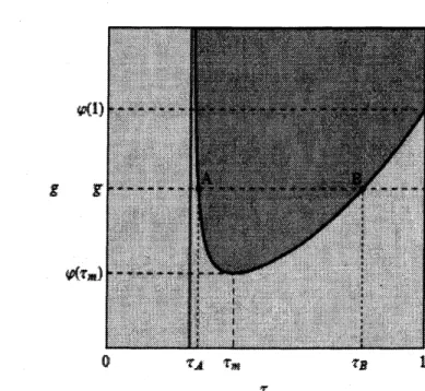
The conditions (ii) and (iii) are visualized in Figure 1. The steady state is

locally stable for all values of the parameters $\tau$ and _$g$ lying in the light-gray

region and locally unstable in the dark-gray region where $1-\alpha\gamma>0,$ $\tau_{-}<$ $\tau<1$ and $g\geq\varphi(\tau)$

.

The division between these two areas is indicated by the

distorted $U$-shaped boundary curve, the locus of$a_{1}a_{2}-a_{0}=0$ or$g=\varphi(\tau)$

.

This

curve separates the stable region from the unstable region in the $(\tau, g)$ plane and

thusoften called thepartition curve. The light-gray region is further divided into

two subregions by the vertical real line $\tau=\tau_{-}$

.

The condition (ii) holds in the

subregion to the left ofthe line andthe steady state is locally stable irrespective

of the value of $g$

.

The condition (iii) holds in the subregion to the right. The

boundary curve, $g=\varphi(\tau)$, is asymptotic to the vertical line as $\tau$ tends to $\tau_{-}$

from

above.2

The minimum value of$\varphi(\tau)$ is attained for _{$\tau=\tau_{m}$}

.

The maximum

value oftax rate $\tau$ is unity by definition and the corresponding value of$\varphi(\tau)$ is

$\varphi(1)$

.

It is then apparent that the horizontal line at $g=\overline{g}$ has no intersection with the partition curve if $\overline{g}<\varphi(\tau_{m})$,

one

intersection if $\overline{g}>\varphi(1)$ and two

intersections including the equal roots otherwise. Notice that $\overline{g}$ is selected so

as to satisfy $\varphi(\tau_{m})<\overline{g}<\varphi(1)$ in Figure 1 and thus the horizontal line

crosses

twice the $g=\varphi(\tau)$ curve at points $A$ and $B$, yielding the corresponding tax

rates $\tau_{A}$ and $\tau_{B}$,

respectively.3

$g$

$\mathfrak{B}$

$\tau_{X}$ $\prime r_{\mathfrak{B}}$ ig $\}$

$\tau$

Figure 1. Stable and instable regions

4

Tax Effect

on

Stability

The $10$cal stability conditions of the steady state are analyticallyobtained. Now

our concern is on global behavior of locally unstable trajectories. The

nonlin-earities of the dynamical system $(M_{I})$ indicates the emergence of limit cycle or

other more complex behavior through a Hopf bifurcation when loss of stability

occurs

on the partition

curve.

Its conditions are as follows:

(Hl) The characteristic equation atthe critical point has apair ofpurely

imag-inary roots and no other roots with zero real parts;

(H2) The real part of these imaginary $ro$ots change $sign$ at the critical point.

Substituting $a_{0}=a_{1}a_{2}$ into equation (4) gives the factored form,

$(\lambda^{2}+a_{1})(\lambda+a_{2})=0.$

On this curve, the characteristic equation has a conjugate pair ofpurely

imagi-nary $ro$ots and one real negative root,

$\lambda_{1,2}=\pm i\sqrt{a_{1}}$ and $\lambda_{3}=-a_{2}<0.$

3The particular values of the paramters to depict Figure 1 are given in the Assumption below.

So

the first condition (Hl) is satisfied. To check the second condition,

we

select the tax rate $\tau$ as the bifurcation parameter and treat the root of the

character-istic equation as a continuous function of $\tau$:

$\lambda(\tau)^{3}+a_{2}\lambda(\tau)^{2}+a_{1}\lambda(\tau)+a_{0}=0.$

Differentiating it with respect to $\tau$ yields

$\frac{d\lambda}{d\tau}=-\frac{\lambda^{2da}\vec{d\tau d_{\mathcal{T}}^{\Delta}}+\lambda\frac{da_{1}}{d\tau}+\underline{d}a}{3\lambda^{2}+2a_{2}\lambda+a_{1}}$

.

Substituting $\lambda=i\sqrt{a_{1}}$and rationalizing the right hand side yield the following

form of the real part of this derivative,

${\rm Re}( \frac{d\lambda}{d\tau}\lambda=i\sqrt{a_{1}})=-\frac{(_{d\tau}^{\underline{d}a}\Delta-a_{1_{\vec{d\tau}}}^{\underline{d}a})(-2a_{1})+2a_{2}a_{1^{\frac{da_{1}}{d\tau}}}}{4a_{1}(a_{1}+a_{2}^{2})}$

.

The denominator is definitely positive. Let

us

denote the numerator as $\Omega$ and

confirm its $sign$. Notice first that

$\Omega=-\frac{2\alpha^{2}\beta^{2}s^{4}(1-\tau)^{2}(Ag\gamma+\mu\tau^{2})}{\tau^{3}A^{6}}\triangle(\tau)$

where

$\Delta(\tau)=-\frac{\mu(1-\tau)\tau^{2}}{\beta\gamma\mu s^{2}(1-\tau)^{2}-(1-\alpha\gamma)\tau A^{2}}\phi(\tau)$

and

$\phi(\tau)$ $=$ $2\beta^{2}\gamma\mu^{2}s^{4}(1-\tau)^{4}-\beta\mu A^{2}s^{2}[1-4\alpha\gamma(1-\tau)-3\tau](1-\tau)\tau$ $-2\alpha(1-\alpha\gamma)A^{4}\tau^{2}.$

Further we have

$\frac{d\varphi}{d\tau}=-\frac{\mu\tau}{Af(\tau)^{2}}\phi(\tau)$

with

$f(\tau)=\beta\gamma\mu s^{2}(1-\tau)^{2}-(1-\alpha\gamma)\tau A^{2}$

Notice that $-f(\tau)$ is the second factor of the denominator of $\varphi(\tau)$

.

Finally $\Omega$

can be expressed as

$\Omega=kf(\tau)\frac{d\varphi}{d\tau}$

with

$k= \frac{2\alpha^{2}\beta^{2}s^{4}(1-\tau)^{2}(Ag\gamma+\mu\tau^{2})(1-\tau)\tau}{\tau^{3}A^{6}}>0.$

Since $\varphi(\tau)$ is defined on the interval $(\tau_{-}, 1)$, we check the $sign$ of $\Omega$ on that

interval. Since,

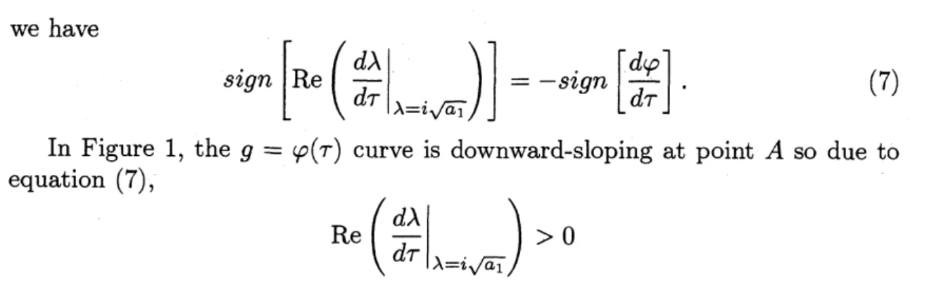
we have

sign $[{\rm Re}( \frac{d\lambda}{d\tau}|_{\lambda=i\sqrt{a_{1}}})]=$ -sign $[ \frac{d\varphi}{d\tau}]$ (7)

In Figure 1, the $g=\varphi(\tau)$ curve is downward-sloping at point $A$ so due to

equation (7),

${\rm Re}( \frac{d\lambda}{d\tau}\lambda=i\sqrt{a_{1}})>0$

implying that all roots cross the imaginary axis at $i\sqrt{a_{1}}$ from left to right as $\tau$

increases, that is, the steady state loses stability. On the other hand, at point

$B$, it is upward-sloping so due to equation (7),

${\rm Re}( \frac{d\lambda}{d\tau}\lambda=i\sqrt{a_{1}})<0$

implying that the steady state regains stability. The effect caused by a change

in the tax rate depends on constellations of $\tau$ and _$g$ and summarized as follows:

Theorem 2 Given $g=\overline{g}$, stability switch occurs twice, to instability

from

sta-bility

_for

$\tau=\tau_{A}$ at point $A$ and to stability

from

instability

for

$\tau=\tau_{B}$ at

point $B$

if

$\varphi(\tau_{m})\leq\overline{g}\leq\varphi(1)$, once

from

stability to instability

if

$\overline{g}>\varphi(1)$ and

no stability switch occurs

_if

$\overline{g}<\varphi(\tau_{m})$ where $\overline{g}=\varphi(\tau_{A})hold_{\mathcal{S}}$ at point $A$ and

$\overline{g}=\varphi(\tau_{B})$ holds at point_$B.$

We numerically examine the analytical results just obtained. Before

pro-ceeding, we specify the parameter values as follows and formulate this selection

as an assumption since we repeatedly use this set of the parameters in further

numerical studies.

Assumption : $\alpha=\beta=A=1,$ $\gamma=4/5,$ $\mu=3,$ $s=1/5$ and $\overline{g}=10.$

Figure 1 is actually illustrated under Assumption and takes the following

parameter values, $\tau_{A}\simeq 0.29,$ $\tau_{B}\simeq 0.8,$ $\tau_{m}\simeq 0.4,$ $\varphi(\tau_{m})\simeq 4.7$ and $\varphi(1)=$

$15$

.

Thus _{$1-\alpha\gamma>0$} and _{$g(\tau_{m})<\overline{g}<g(1)$}. According to Theorem 2, the

stationary state of the $3D$ system $(M_{I})$ loses local stability at point $A$ and

regains it at point $B$

.

Local stability does not necessarily mean global stability

in a nonlinear system. To find how nonlinearities in system $(M_{I})$ affect global

dynamics, we _{numerically detect the effects caused} by a change in the tax rate

on global dynamics between $\tau_{A}$ and $\tau_{B}$

.

In performing simulations, we take

the same initial values for $Y(O)=Y^{*}$ and $R(O)=R^{*}$ and the different initial

values of $M(O),$ $M(O)=M^{*}+1$ _{in the first simulation and $M(O)=M^{*}+5$}

in the second simulation. The resultant bifurcation diagrams are presented in

Figures 2(A) and (B), in each of which thedownward sloping blackcurvedepicts

the equilibrium value of output, $Y^{*}=g/\tau$

.

In the simulations, the bifurcation

parameter$\tau$is increased from 0.2to 1withanincrement of1/1000,theiterations

last

100

iterations

are

plotted against each value of $\tau$. In Figure 2(A), the

bifurcation diagram of the first simulation is depicted. It is observed that the

stationary state loses stability when $\tau$ arrives at $\tau_{A}$

and

bifurcates to aperiodic

cycle having

one

maximum and one minimum for $\tau>\tau_{A}$

.

It is also observed

that

an

oscillation disappears at $\tau=\tau_{B}$ and stability is regained for $\tau>\tau_{B}$

.

In

Figure 2(B), the bifurcation diagram in the second simulation is illustrated. It

is seen that stability is lost at $\tau=\tau_{A}$

as

in Figure 2(A) but regained at

some

value larger than $\tau_{B}$

.

Further simulations with different initial points have been

conducted and then lead to the fact that stability is regained not necessarily at

$\tau=\tau_{B}$ but at

some

larger value although stability is always lost at $\tau=\tau A.$

This difference implies that it depends on a selection of the initial values of the

variables when it regains

stability.4

These numerical results are summarized

as

follows:

Proposition 3 The. nonlinear $IS$-$LM$ model $(M_{I})$ generates periodic

oscilla-tions when the steady state is destabilized and has initial point dependency to

regain stability.

$\tau_{A} \tau,$

_{$\tau_{l} \{r_{\delta}$}

$\tau$

$\tau$

(A) $M(0)=M^{*}+1$ _{(B) $M(0)=M^{*}+5$}

Figure 2. Bifurcation diagrams with different initial values

De Cesare and Sportelli (2005) and Fanti and Manfredi (2007) also examine

the local stability and arrive at the same result

as

in Theorem 1. However, the

former does not consider a Hopf bifurcation in the undelay model whereas the

latter discusses the Hopf bifurcation with respect to the government

expendi-ture, the other fiscal policy parameter, but not with respect to the tax rate. As

can be

seen

in Figure 1, given

,

increasing $g$ destabilizes the steady

state when it crosses the partition curve from below. As a natural consequence,

neither authors mention a possibility of stability regain with respect to the tax

rate.

References

[1] De Cesare, L. and Sportelli, M. (2005): A Dynamic $IS$-LM model with

Delayed Taxation Revenues, Chaos, Solitions and Fractals, 25, 233-244.

[2] Fanti, L. and Manfredi, P. (2007): ChaoticBusiness Cyclesand Fiscal Policy:

An $IS$-LMModel with Distributed Tax Collection Lags, Chaso, Solitions

and Enactals, 32, 736-744.

[3] Gandolfo,

G.

(2010): Economic Dynamics, 4th Edition, Springer-Verlag,

Berlin/Heiderberg/New York.

[4] Goodwin, R. (1951): TheNonlinear Accelerator and the Persistence of

Busi-ness Cycles, Econometrica, 19, 1-17, 1951.

[5] Kalecki, M., A. (1935): Macrodynamic Theory of Business Cycles,

Econo-metrica, 3, 327-344.

[6] Sasakura, K. (1994): On the Dynamic Behavior ofSchinasi’sBusiness Cycle

Model, Journal of Macroeconomics, 16, 23-444.

[7] Schinasi,

G.

(1982): Fluctuations in a Dynamic, Intermediate-run $IS$-LM

model: Applications of the Poincare-BendixsonTheorem, Journalof

Eco-nomic Theory, 28,

369-375.

[8] Matsumoto, A. and Szidarovsky, F. (20013): Dynamics in Delay $IS$-LM