九州大学学術情報リポジトリ

(1)

九州大学学術情報リポジトリ

Kyushu University Institutional Repository

埋込み境界法を用いた流れと複雑・移動境界の干渉に関する流体現象の数値解析的研究

张 , 晏榕

http://hdl.handle.net/2324/1959133

出版情報：Kyushu University, 2018, 博士（工学）, 課程博士バージョン：

権利関係：

(2)

Numerical study of flow phenomena concerning interaction of flow and complex or moving boundaries using immersed boundary method

Yanrong Zhang

Department of Aeronautics and Astronautics Kyushu University

July, 2018

(3)

List of figures

Figure 3.1: The category of the cell structures………24

Figure 3.2: Schematic pictures of cell-center method and vertex-center method…………24

Figure 3.3: Schematic computational procedure of FrontFlow/red………25

Figure 3.4: Schematic computational procedure including the IB mechanism…………...25

Figure 3.5: Schematic computational procedure including the IB and feedback mechanism……….26

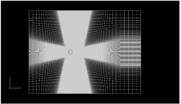
Figure 4.1: Grid plane perpendicular to the spanwise direction: entire view (upper) and partial magnification near the cylinder (lower).………..45

Figure 4.2: Schematic diagram of the single particle settling………46

Figure 4.3: Grid (coarse) and roughness (fine)………...47

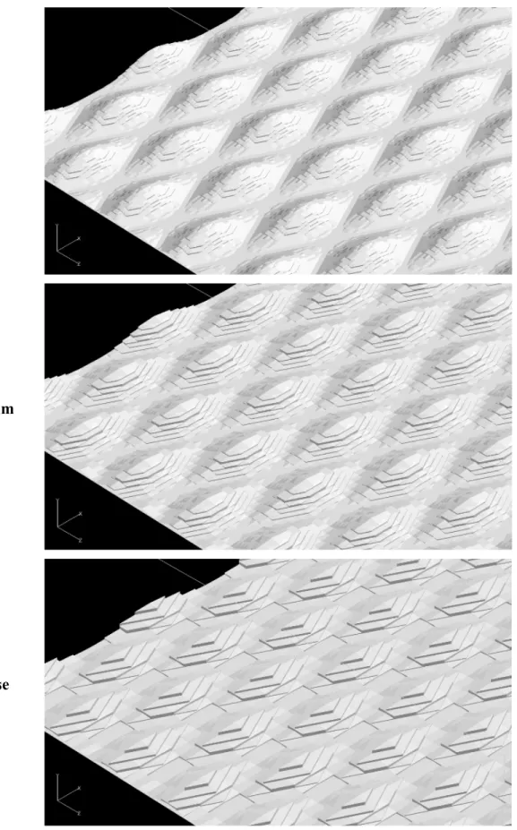
Figure 4.4: Close-up views of the three rough bottom surfaces……….48

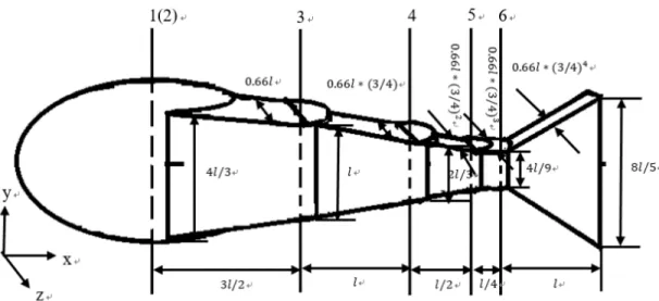
Figure 4.5: Computational model and dimensions (𝑙𝑙= 0.15)………49

Figure 4.6: Body-fixed coordinate systems………49

Figure 4.7: (a) Definition of the kinematics (top view); (b) Schematic postures in a tail- beat cycle for different phase differences (𝐴𝐴= 1/4)……….50

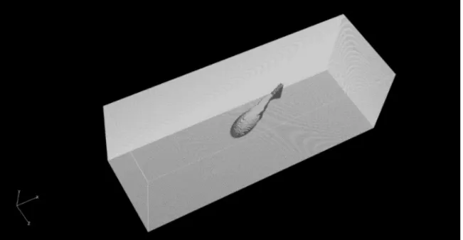
Figure 4.8: Grid for the simulation……….51

Figure 5.1: Lift and drag coefficients against time for Re = 100 (upper) and 1000 (lower)………66

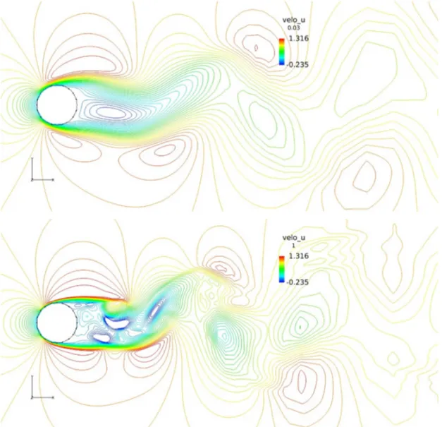
Figure 5.2: Instantaneous streamwise velocity contours on the center plane for Re=100 (upper) and 1000 (lower)………...67

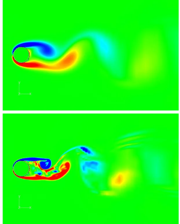
Figure 5.3: Vorticity contours on the center plane for Re=100 (upper) and 1000 (lower), where blue for clockwise and red for counter-clockwise………68

Figure 5.4: Vortex structures for the case of Re=1000………69

Figure 5.5: Velocity profiles for a single settling particle……….69

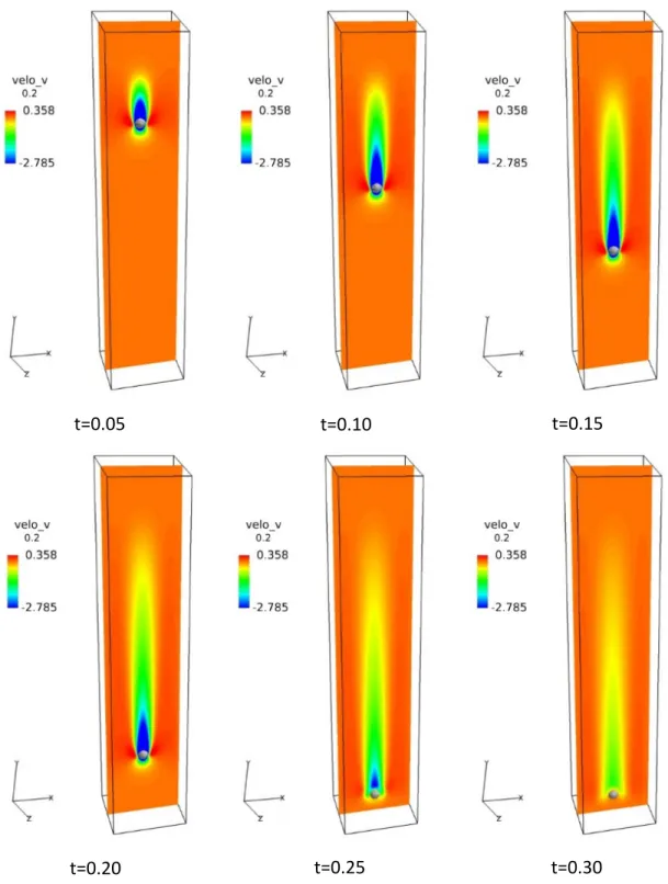
Figure 5.6: Color contours of velocity on the central plane………70

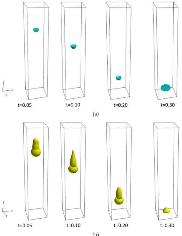
Figure 5.7: Vortex structures around the settling particle with second invariant of the velocity-gradient tensor of (a) 10 and (b) -20………71

Figure 5.8: Velocity profiles for a single settling particle with different time steps………72 III

(6)

Figure 5.9: Longitudinal displacement (upper) and velocity (lower) against time for the cases with different time steps or grids (A=0.25, ω= π , ϕ=π/

6)………73

Figure 5.10: Mean streamwise velocity for the smooth wall………...74

Figure 5.11: Comparison of Reynolds stresses for flow along a smooth wall………75

Figure 5.12: Comparison of the mean streamwise velocity for rough-wall cases with smooth-wall DNS………...77

Figure 5.13: Instantaneous velocity with roughness shape at z=0 (with EAT)…………..78

Figure 5.14: Comparison of turbulence energy distributions……….79

Figure 5.15: Comparison of Reynolds stress for the rough-wall cases and DNS cases (smooth and rough)………80

Figure 5.16: SGS components of the Reynolds stresses for the coarse case………82

Figure 5.17: Comparison of the Reynolds shear stress………...83

Figure 5.18: Comparison of the turbulence energy……….86

Figure 5.19: Instantaneous vortex structures and streamwise velocity (4.8, 0.02, 0) contours (with EAT)……….89

Figure 5.20: Displacement and velocity component against time along the three directions for cases with different angular velocities (ϕ=𝜋𝜋/6 and A=0.25)……...90

Figure 5.21: Velocity vectors and color contours for cases with different angular velocities (𝜙𝜙 =𝜋𝜋/6 and A=0.25)………...93

Figure 5.22: Vortex structures for cases with different angular velocities (𝜙𝜙 = 𝜋𝜋/6 and A=0.25)………..95

Figure 5.23: Velocity vectors and color contours of velocity in one cycle for the case of ω=π with ϕ=𝜋𝜋/6 and A=0.25……….97

Figure 5.24: Vortex structures visualised according to the second invariant of the velocity- gradient tensor in one cycle for ω=π with ϕ=𝜋𝜋/6 and A=0.25………98

Figure 5.25: Pressure distribution on the surface in one cycle for case of ω=π with ϕ= 𝜋𝜋/6 and A=0.25……….99

Figure 5.26: Profiles of the displacement and velocity component against time along three directions for different phase differences (ω= π and A=0.25)………100

IV

(7)

Figure 5.27: Velocity vectors and color contours for cases with different phase difference

(ω= π and A=0.25)……….103

Figure 5.28: Vortex structures for ω=π and A=0.25……….105 Figure 5.29: Displacements and velocity components against time along three directions for the cases with different body amplitudes ( ω= π and ϕ=π/

6)………..107 Figure 5.30: (a) Enlarged profiles of the longitudinal velocities for the cases with different amplitudes (ω= π and ϕ= π/6); (b) Postures of the fish model in one tail-beat cycle for the case of A=0.3 (ω= π and ϕ= π/6)………110 Figure 5.31: Velocity vectors and color contours for cases with different body amplitudes

(ω= π and ϕ= π/6)………..111

Figure 5.32: Vortex structures for cases with different body amplitudes (ω=π and ϕ= π/6)………..113 Figure 5.33: Profiles of displacements and velocity components against time along three directions for the cases using grids of different widths……….115 Figure 5.34: Profiles of displacements and velocity components against time along three directions for the cases using grids of different heights………118

V

(8)

List of tables

Table 1.1 Eulerian, Lagrangian and ALE methods ………..3 Table 4.1: Grids for the three test resolutions with roughness……….36 Table 4.2: Formula for inside-outside judgement………...41 Table 5.1: Comparison of drag coefficient and Strouhal number with those in previous studies………52 Table 5.2: Comparison of the limit velocity with previous studies……….53 Table 5.3: Computational cost for the rough-wall cases……….60

VI

(9)

Nomenclature

a Constant

𝑎𝑎⃑ Acceleration of the model 𝑎𝑎_𝑓𝑓

��⃑ Acceleration of fluid

𝐴𝐴 Undulatory amplitude

𝐴𝐴_𝑐𝑐 Reference area

𝐴𝐴0 Modelling parameters

b Constant

𝑏𝑏_{𝑖𝑖𝑖𝑖}^{𝑆𝑆𝑆𝑆𝑆𝑆} Anisotropy tensor

c Constant

𝑐𝑐_𝑠𝑠 Size parameters of the fish model Cl Lift coefficient

Cd Drag coefficient

𝐶𝐶𝐵𝐵, 𝐶𝐶_{𝑆𝑆𝑆𝑆𝑆𝑆}, 𝐶𝐶_𝑙𝑙, 𝐶𝐶_𝜀𝜀, 𝐶𝐶_𝑘𝑘 Modelling parameters

D Diameter of circular cylinder in validation case

𝑓𝑓⃑ Body force

𝑓𝑓_𝑠𝑠

��⃑ Surface force

𝐹𝐹⃑ External force

𝐹𝐹_𝑑𝑑 Drag force

𝐹𝐹_𝑙𝑙 Lift force

ℎ Roughness height from peak to valley 𝚤𝚤 �⃑, 𝚥𝚥 ��⃑, 𝑘𝑘 ��⃑ Unit vectors of the inertia coordinate system 𝚤𝚤_𝑠𝑠

��⃑, 𝚥𝚥��⃑, 𝑘𝑘_𝑠𝑠 ��⃑_𝑠𝑠 (s=1,2,…,7) Unit vectors of the body-fixed coordinate system (s) [𝐼𝐼_𝑅𝑅] Inertia matrix

𝐼𝐼 Constants

𝑙𝑙 Size parameters of the fish model

𝑙𝑙𝑥𝑥, 𝑙𝑙𝑧𝑧 Wavelengths of the roughness element in x- and z- directions

VII

(10)

𝑘𝑘𝑆𝑆𝑆𝑆𝑆𝑆 SGS turbulent kinetic energy (SGS turbulence energy) 𝑚𝑚 Setting mass of the model

𝑛𝑛�⃑ Wall normal unit vector

𝑝𝑝 Pressure

𝑟𝑟_1𝑥𝑥, 𝑟𝑟_1𝑦𝑦, 𝑟𝑟_1𝑧𝑧 Coordinates of the origin point of the body-fixed coordinate system (1) in the inertia coordinate system 𝑟𝑟⃑ Location vector in the inertia coordinate system 𝑟𝑟1

��⃑ Location vector of the origin point of the body-fixed

coordinate system (1) in the inertia coordinate system 𝑟𝑟_𝑐𝑐

��⃑ Location vector of the center of mass of the model in the inertia coordinate system

𝑟𝑟_𝑛𝑛

��⃑ Vector from the origin of 𝑛𝑛�⃑ to the point to be identified 𝑟𝑟𝑜𝑜1

��⃑ Location vector in the body-fixed coordinate system (1)

𝑅𝑅 Size parameters of the fish model

𝑅𝑅𝑅𝑅 Reynolds number

RHS Right-hand side

𝑆𝑆𝑖𝑖𝑖𝑖 Resolved strain-rate tensor

St Strouhal number

𝑡𝑡 Time

Δt Scale of time step

𝑇𝑇�⃑ External torque

T Temperature

𝑢𝑢�⃑ Velocity

𝑢𝑢�⃑𝑏𝑏 Velocity inside the immersed boundary 𝑢𝑢_𝑠𝑠

��⃑ Velocity of the origin point of the body-fixed coordinate

system (s) 𝑢𝑢_Γ

��⃑ Velocity at the immersed boundary

𝑢𝑢_𝜏𝜏 Friction velocity

𝑢𝑢𝑖𝑖 Velocity component in i direction VIII

(11)

𝑢𝑢_𝑖𝑖^𝑛𝑛+1, 𝑢𝑢_𝑖𝑖^𝑛𝑛 Velocity at node i at time step n+1, n 𝑈𝑈_𝑖𝑖 Velocity component in i-direction 𝑈𝑈∞ Far field velocity

𝑉𝑉�⃑_{𝑖𝑖𝑏𝑏} Desired velocity inside the immersed boundary x, y, z Coordinates in the inertia coordinate system

𝑥𝑥_𝑖𝑖 Cartesian coordinate in i-direction

𝑥𝑥1, 𝑦𝑦₁, 𝑧𝑧₁ Coordinates in the body-fixed coordinate system (1) 𝛼𝛼⃑ Angular acceleration of the model

µ Molecular viscosity

𝜌𝜌 Density

𝜌𝜌_𝑓𝑓 Density of fluid

ν Kinematic viscosity

Δ SGS filter width

δ Open-channel height

𝛿𝛿_{𝑖𝑖𝑖𝑖} Kronecker delta

𝜎𝜎0 Mean offset

𝜈𝜈_{𝑆𝑆𝑆𝑆𝑆𝑆} SGS eddy viscosity

𝜀𝜀𝑆𝑆𝑆𝑆𝑆𝑆 Dissipation rate of SGS turbulence energy

𝜏𝜏𝑖𝑖𝑖𝑖 SGS-stress tensor

Γ_𝑏𝑏 Immersed boundary

Ω_𝑏𝑏 Field inside the body Ω_𝑓𝑓 Field of the fluid

Ω𝑏𝑏 Field inside the immersed boundary 𝜔𝜔 Undulatory angular velocity

𝜔𝜔��⃑ Angular velocity of the model

𝜔𝜔_𝑠𝑠

��⃑ Angular velocity of the body-fixed coordinate system (s)

𝜙𝜙 Phase difference between the neighboring parts of the model

(. . )

�� Filtered value

IX

(12)

(. . )� Test-filtering operator

X

(13)

Chapter 1 Introduction

1.1 About the boundary methods in computational fluid mechanics

Complicated or moving boundaries are common in normal life as well as various engineering applications. For example, free surface of the sea, flapping wings of a bird or beating tail of a fish and rotational propeller of an aircraft. Owing to the development of the computer technique, computational fluid dynamics (CFD) is becoming more and more important to study various flow phenomena in addition to the experiment. To perform the computational simulation for the problems concerning complicated or moving boundaries, dealing with the boundaries is a crucial point.

The treatment of the boundary in simulation is based on the scheme by which the movement of fluid is described. To describe the movement of fluid mathematically, there are the Eulerian method and the Lagrangian method as two different approaches. In the Eulerian method, the flow is expressed as a field in which observing points are fixed inside.

By obtaining the physical quantities such as the velocity of fluid instantaneously passing these observing points, the movement of fluid is clarified. In the Lagrangian method, on the other hand, the flow field is not fixed, the flow is expressed by tracing the movement of fluid particles. Generally, in the numerical simulation of fluid flow, the Eulerian method is more popular than the Lagrangian method. While when there is free surface or moving boundary in a flow field, the Lagrangian method is also frequently used. Before simulation, it is necessary to discretize the simulation field, for example the structured meshes in the finite difference method. In the Eulerian approach, the discretized meshes are fixed during the simulation and the grid vertices could be regarded as the observing points for a flow.

While in the Lagrangian approach, the grid vertices could be regarded as corresponding to fluid particles, thus could be made to move with the fluid particles. Therefore, the movement of a free surface or a moving boundary could not be directly captured by using the Eulerian approach and some additional processes to describe the movement of boundary need to be introduced. In contrast to this, in the Lagrangian approach, since the grid vertices are considered as the fluid particles, the moving boundary could be directly captured by tracing the grid vertices corresponding to the moving boundary. However, as

1

(14)

the grid vertices move, remeshing is needed at each time step during the simulation, when in case of such as surface with large vibration or breaking wave, large movement of the corresponding grid vertices arises and the computation may be unavailable because of the collapsing of the mesh (数値流体力学編集委員会,1995). To improve this drawback of the Lagrangian method, Arbitrary Lagrangian-Eulerian (ALE) method was proposed. In the ALE, the moving velocity of the mesh that is independent of the velocity of the corresponding fluid particles is employed to prevent an excessive deformation of the mesh.

To achieve that, a referential description of the fundamental equations is required. A conclusion about the properties of the ALE method as well as the Eulerian and Lagrangian methods is listed in Table 1.1.

Although describing the moving boundary by the Lagrangian and ALE methods is relatively straightforward, both of them need the remeshing during simulation. By using the Eulerian method, the remeshing could be avoided while additional processes are required to describe the moving boundary indirectly, such as height function, line segment, marker particle, density function and so on. Since by the Eulerian method the description of the moving boundary is not constrained by the mesh, it is relatively easier to deal with large deformation. However, the accuracy of computation is said to be generally lower due to a lower level of satisfaction of conservation near a moving boundary (数値流体力学編集委員会, 1995）.

Among such several strategies, the immersed boundary method that belongs to the Eulerian approach is a promising approach to deal with the complicated or moving boundary problems in CFD, in which the effect of a boundary is imposed by introducing an extra force into a fluid flow. Remarkable development has been made since it was proposed and numerous applications have been performed. While despite of the obtained achievement, applications of the immersed boundary are found usually confined to the problems with relatively low Reynolds numbers or relatively simple movement, applications including moving boundary with relatively complicated configuration or self-induced movement is also limited. The difficulty of obtaining a boundary layer accurately and describing the moving boundary in an unbody-fitted mesh is considered as one of the main reasons.

2

(15)

Table 1.1 Eulerian, Lagrangian and ALE methods (数値流体力学編集委員会, 1995） Method Velocity of

mesh (𝑣𝑣�⃑) and fluid (𝑣𝑣⃑)

Properties

Eulerian method

𝑣𝑣�⃑ = 0

Computational mesh is fixed spatially;

Additional process is needed for moving boundary;

Algorithm is relatively simple because of no remeshing.

Lagrangian method

𝑣𝑣�⃑= 𝑣𝑣⃑

Computational mesh moves corresponding to the velocity of fluid particles;

Description of the moving boundary is relatively simple, the distortion of mesh becomes serious in case of large movement;

Remeshing is required on each time step.

ALE (Arbitrary Lagrangian-

Eulerian method)

𝑣𝑣�⃑ ≠ 𝑣𝑣⃑

Computational mesh could move independently to the velocity of fluid particles;

Description of the moving boundary is relatively simple, the distortion of mesh could be adjusted during simulation;

Remeshing could be implemented only in the vicinity of moving boundary, thus relatively less cost is required.

1.2 About the simulation of turbulence

For engineering applications, the flows are mostly turbulent and they are highly unsteady in time and contain numerous vortices with the scales spanning widely. Generally, the turbulence energy transfers from large vortices to small ones and dissipate into heat at last.

To generate the vortices of all scales, it is generally said that a grid number of 𝒪𝒪[𝑅𝑅𝑅𝑅^9/4] is necessary. Except for few limited cases, it is difficult to simulate all the vortices by using the capability and memory of current computers. Besides that, issues such as the

3

(16)

preparation of initial conditions, discretization error and the chaos from the nonlinear make the accurate prediction of turbulence flow more impossible (梶島岳夫,1999).

Methods to carry out the simulation of turbulent flows include direct numerical simulation (DNS), large-eddy simulation (LES) and Reynolds-averaged Navier-Stokes simulation (RANS). For the DNS, the equations are discretized directly without performing any turbulence model, all vortices are supposed to be calculated directly. Because of an extremely high computational cost, DNS is usually used for obtaining basic data of turbulent flow phenomena, while for many engineering applications that are frequently turbulent at high Reynolds numbers, implementing DNS is quite difficult, although DNS has provided valuable results (for example, Moser, Kim, &Mansour, 1999) and is proved to be an effective method to investigate the turbulence besides the experiment. For the LES, on the other hand, only relative large eddies are computed while the effect of small ones is modeled. Filter function is employed to build the equations for discretization. The filter scale is usually set to be the same as the grid scale, thus the vortices are divided into the grid scale (GS) that is to be computed and the subgrid scale (SGS) that is to be modeled.

The modeling methods for LES include the Smagorinsky model, the scale similarity model, the dynamic Smagorinsky model and so on. For the RANS, all vortices are modeled, the Reynolds averaging is implemented on the equations and the resulting unknown terms such as the Reynolds stress or diffusion flux in the Reynolds stress equations are closed by modeling. The eddy-viscosity model or the Reynolds stress equation model is adopted in the RANS calculation. Numerous achievements have been made on developing modeling methods for simulation of turbulence, however universal model that can be applied to every turbulent flow is still lacked (梶島岳夫, 1999).

1.3 Objectives of the present study

In the present study, applications of the immersed boundary method on the problems concerning rough or moving boundaries are carried out. For this purpose, a force feedback mechanism is added to an original program code “FrontFlow/Red” (小林敏雄, 2004; 畝村毅, 2003; Muto, Tsubokura, & Oshima, 2012; http://www.ciss.iis.u-tokyo.ac.jp/rss21/) that is introduced in Chapter 3 to simulate the movement in flow controlled by the

4

(17)

hydrodynamic force. The performance of the immersed boundary method including the feedback mechanism is validated firstly and three-dimensional flow phenomenon in the interaction of the fluid and boundary is investigated, the present test cases include:

1. Validation case for the static immersed boundary: flow around a circular cylinder.

Two cases with Reynolds number at 100 and 1000 are carried out, respectively. The obtained results are compared with those of other previous studies.

2. Validation case for the moving boundary involving the force feedback: single settling sphere particle in fluid. A sphere particle is set free statically and falls under the gravity effect and reaches a limit velocity when the gravity is balanced with the drag and buoyancy. The obtained results are compared with those of other previous studies.

3. Application of the immersed boundary method to build the rough structure in the study on the effect of an anisotropy-resolving subgrid-scale model on large eddy simulation predictions of turbulent open channel flow with wall roughness. The roughness on the bottom surface of channel is defined using the ‘egg-carton’ shaped- surface function (Bhaganagar et al., 2004). Grid dependency of the turbulence model (Abe, 2013) on the flow prediction near the rough surface is investigated in detail.

4. Three-dimensional simulation of a self-propelled fish-like body swimming in a channel where the fish model and movement are defined in a structured grid using the immersed boundary method. To satisfy the continuity inside the immersed boundary, a rigid-body system is adopted to build the fish model. A parametric study of kinematic factors is performed to study the hydrodynamics in fish swimming.

An introduction about the immersed boundary method is given in Chapter 2. Numerical simulation method is provided in Chapter 3. The details of the present computational cases are introduced in Chapter 4. The results are then discussed in Chapter 5, and the conclusions of the study are drawn in Chapter 6.

5

(18)

Chapter 2 Immersed boundary method

2.1 Introduction

As aforementioned, with applying the immersed boundary (IB) method, there is no need to modify the grid when carrying out the simulation with moving boundary, thus the corresponding computational time of remeshing can be saved. This is a considerable advantage especially when there is large displacement. The IB method is considered firstly to be proposed by Peskin (1972) to study the flow around heart valves where the boundary was replaced by a force and a semi-discrete analog of the δ function is introduced to link the representation of the boundary and fluid. An extending numerical study including the muscular heart wall was also carried out (Peskin, 1977). By now, many studies have been performed on this method as follows for examples. Iaccarino and Verzicco (2003) reported some results on the application of the IB method for turbulent flow simulations using both RANS and LES. Details of forcing definition and boundary treatment were illustrated.

Tseng and Ferziger (2003) presented a second-order ghost-cell immersed boundary method for turbulent flows in complex geometries. In the study, the ease of implementation of this method in existing codes was demonstrated and the obtained computational results agreed well with the previous experimental and numerical results. Noor, Chern and Horng (2009) presented a direct-forcing IB technique to solve fluid-solid interaction problems. Taira and Colonius (2007) presented a formulation of the IB method modeled algebraically identical to the traditional fractional step method to simulate the flows over bodies with prescribed motion. In the study, regularization and interpolation operators were introduced to satisfy the no-slip constraint on the immersed surfaces, and the boundary force was regarded as the Lagrange multiplier like pressure. Slip and non-divergence-free components of the velocity field were removed by a projection in the approach. Fadlun et al. (2000) showed the effect of the interpolation of forcing over a grid on the accuracy of the scheme and applied the IB method to the flow inside an IC piston/cylinder assembly at high Reynolds number. Goldstein, Handler and Sirovich (1993) simulated the no-slip flow boundary using the IB method and determined the needed surface body force by a feedback scheme in which the velocity is used to build the formula. Balaras (2004) presented a method based

6

(19)

on the direct forcing approach to carry out LES around complex boundaries on fixed Cartesian grids. In the study, a novel interpolation scheme and a method to deal with SGS fluxes near the interface were introduced. Abundant developments show the IB method a promising way to deal with complex and moving boundaries.

2.2 Category of the immersed boundary method

When applying the IB method, in general, the effect of the boundary on a flow is realized by imposing a body force through some forcing functions. Besides this, there is also another approach: the so-called cut-cell approach, in which new cells that conform to the shape of a body is generated by truncating the Cartesian cells at the immersed boundary (Bandringa, 2010). For the first approach, the Navier-Stokes equation for an incompressible viscos flow including the body force is as follows (Hirose, 2013):

𝜌𝜌 �^{𝜕𝜕𝑢𝑢��⃑}_{𝜕𝜕𝜕𝜕}+𝑢𝑢�⃑ ∙ ∇𝑢𝑢�⃑�+∇𝑝𝑝 − 𝜇𝜇∆𝑢𝑢�⃑ =𝑓𝑓⃑, (2.1)

∇ ∙ 𝑢𝑢�⃑= 0 in Ω_𝑓𝑓 and (2.2) 𝑢𝑢�⃑ =𝑢𝑢��⃑ on Γ_Γ _𝑏𝑏. (2.3)

Where 𝑓𝑓⃑ is the body force, 𝜌𝜌 is the density, 𝜇𝜇 is the kinematic viscosity, 𝑢𝑢�⃑ and 𝑝𝑝 are the velocity and the pressure, respectively. Γ_𝑏𝑏 denotes the boundary, Ω_𝑏𝑏 and Ω_𝑓𝑓 are the field of body and fluid, respectively, which are divided by the boundary Γ_𝑏𝑏.

To calculate the body force, various methods have been proposed as shown in Iaccarino,

& Verzicco (2003). The body-force functions can be generally divided into the continuous forcing and the discrete forcing approach (Mittal, & Iaccarino, 2005).

By using the continuous forcing approach, it is straightforward to insert a computing unit into an original program because it is independent of the spatial discretization. While smoothing of the forcing function causes unavailability of the sharp representation of the immersed boundary, which makes the continuous forcing approach not suitable for high Reynolds number flows (Bandringa, 2010). Also, with increasing Reynolds numbers, the proportion of the grid nodes inside the immersed boundary that require to solve the

7

(20)

governing equations increases, this lowers the computational efficiency. Many applications of the methods belonging to this category are found in biological and multiphase flows where elastic boundaries are usually seen, for which the continuous forcing approach is attractive. While there are some challenges for applying this approach to flows with rigid boundaries for the forcing terms generally do not work well in the rigid limit (Mittal et al.

2005).

The direct forcing approach was reported (Fadlun et al., 2000; Balaras, 2004) firstly introduced by Mohd-Yusof (1997). In contrast to the continuous forcing approach, a sharp representation of the immersed boundary can be made by the direct forcing approach, which is necessary for high Reynolds number flows. Without using specified parameters in the forcing, no extra stability constraints are introduced for the immersed boundary (Bandringa, 2010). While the forcing procedure of this approach is highly associated with the discretization and the implementation is not as straightforward as the continuous forcing approach, the inclusion of the boundary motion could be more difficult (Mittal, 2005).

In the present study, the direct forcing approach is adopted to perform the simulations of flows with immersed boundaries inside because of its advantages such as the capability of a sharp representation of boundary that is required in some following cases where the Reynolds number may be relatively high. The immersed bodies could be static or moving in setting modes, and by introducing some feedback mechanism, movement in flow induced by the hydrodynamic force can also be simulated. An introduction of the direct forcing approach is given in Section 2.3.

2.3 Direct forcing approach

The non-dimensional incompressible Navier-Stokes equations including the body force 𝑓𝑓⃑

is as follows (Hirose, 2013):

𝜕𝜕𝑢𝑢��⃑

𝜕𝜕𝜕𝜕+𝑢𝑢�⃑ ∙ ∇𝑢𝑢�⃑+∇𝑝𝑝 −_{𝑅𝑅𝑅𝑅}¹ ∆𝑢𝑢�⃑= 𝑓𝑓⃑, (2.4)

∇ ∙ 𝑢𝑢�⃑= 0 in Ω_𝑓𝑓 and, (2.5) 8

(21)

𝑢𝑢�⃑ =𝑢𝑢��⃑ on Γ_Γ _𝑏𝑏. (2.6) To avoid any misunderstanding, it is noted that the denotations that are the same as those in Section 2.2 mean the non-dimensional values here.

The time discretization form of Eq. (2.4) is as:

𝑢𝑢_𝑖𝑖^𝑛𝑛+1−𝑢𝑢_𝑖𝑖^𝑛𝑛

Δ𝜕𝜕 =𝑅𝑅𝑅𝑅𝑆𝑆_𝑖𝑖+𝑓𝑓_𝑖𝑖, (2.7) where the superscript denotes the time step and subscript denotes the spatial nodes, and 𝑅𝑅𝑅𝑅𝑆𝑆_𝑖𝑖 =−𝑢𝑢�⃑ ∙ ∇𝑢𝑢�⃑ − ∇𝑝𝑝+_{𝑅𝑅𝑅𝑅}¹ ∆𝑢𝑢�⃑. Let 𝑉𝑉_{𝑖𝑖𝑏𝑏}^𝑛𝑛+1 is the desired velocity at n+1 step inside the immersed boundary, the body force 𝑓𝑓_𝑖𝑖 could then be obtained as:

𝑓𝑓_𝑖𝑖 =^𝑉𝑉^{𝑖𝑖𝑖𝑖}^𝑛𝑛+1_∆𝜕𝜕^−𝑢𝑢^𝑖𝑖^𝑛𝑛− 𝑅𝑅𝑅𝑅𝑆𝑆_𝑖𝑖. (2.8)

Outside the immersed boundary, there is no body force. The calculation of body force 𝑓𝑓⃑ is concluded as:

𝑓𝑓⃑=�(𝑢𝑢�⃑ ∙ ∇)𝑢𝑢�⃑+∇𝑝𝑝 −_{𝑅𝑅𝑅𝑅}¹ ∆𝑢𝑢�⃑+_∆𝜕𝜕¹ �𝑉𝑉��⃑ − 𝑢𝑢�⃑𝚤𝚤𝑏𝑏 ^𝑛𝑛�, 𝑛𝑛𝑅𝑅𝑎𝑎𝑟𝑟 Γ𝑏𝑏 𝑜𝑜𝑟𝑟 𝑖𝑖𝑛𝑛 Ω𝑓𝑓

0, 𝑅𝑅𝑙𝑙𝑒𝑒𝑅𝑅𝑒𝑒ℎ𝑅𝑅𝑟𝑟𝑅𝑅. ; (2.9)

The detailed computational procedure is as (Balaras, 2004):

1. Calculate the intermediate 𝑢𝑢�⃑^∗ by the discretized Navier-Stokes equations without considering the body force term. The obtained 𝑢𝑢�⃑^∗ does not fulfill the IB boundary condition.

2. Calculate 𝑓𝑓⃑^𝑛𝑛+1 by Eq. (2.9). The body force could be imposed on the grid nodes in the vicinity of the immersed boundary or all inside. The desired velocity 𝑉𝑉��⃑_{𝚤𝚤𝑏𝑏} could be determined straightforwardly or through interpolation approaches depending on the location of node.

9

(22)

3. Calculate the new 𝑢𝑢�⃑^∗ by the Navier-Stokes equations including the body force term, this new velocity fulfills the IB boundary condition.

4. Calculate the pressure by Poisson equation.

5. Update the velocity and pressure.

6. Go back to step 1.

By setting different desired velocity (𝑉𝑉_{𝑖𝑖𝑏𝑏}^𝑛𝑛+1) field, different boundary conditions can be yielded. Noted that although the fluid inside the immersed boundary is regarded as a “body”

part in computations, it is still controlled by the continuity equation, therefore the desired velocity field should be chosen properly. If the desired velocity field does not satisfy the continuity condition, the calculation may not go well for some undesirable flow flux may arise on the boundary if the flow is incompressible. Considering this constraint, the desired velocity field is set as certain velocity field in a rigid body system for simplicity in the present study. For example, 𝑉𝑉_{𝑖𝑖𝑏𝑏}^𝑛𝑛+1 = 0 corresponds to a static boundary or body; 𝑉𝑉_{𝑖𝑖𝑏𝑏}^𝑛𝑛+1 = 𝑉𝑉0 corresponds to a translational boundary or body; and 𝑉𝑉_{𝑖𝑖𝑏𝑏}^𝑛𝑛+1 = 𝜔𝜔0𝑟𝑟 corresponds to a rotational boundary or body. Combination of these movement is also available. The definition of desired velocity field for different cases may change depending on the computational goals and is illustrated in Chapter 4.

10

(23)

Chapter 3 Numerical simulation method

3.1 Solver of simulation

The simulation in the present study is performed using the open-source-computational fluid dynamics (CFD)-code “FrontFlow/Red” (小林敏雄, 2004; 畝村毅, 2003; Muto, Tsubokura, & Oshima, 2012; http://www.ciss.iis.u-tokyo.ac.jp/rss21/), which is exploited in the project of “Revolutionary Simulation Software” (http://www.rss21.iis.u-tokyo.ac.jp/) having started in 2005 as a part of the next-generation IT program sponsored by the Ministry of Education, Culture, Sports, Science and Technology (MEXT).

3.1.1 Fundamental equations (小林敏雄, 2004)

The present software mainly deals with flows that are at low Mach number and incompressible, although computations concerning compressible flow is also possible in principle. Here, the mass-conservation and momentum-conservation equations involved in the present study are illustrated as follows.

Mass conservation equation

The mass conservation equation is as follows:

𝜕𝜕𝜕𝜕

𝜕𝜕𝜕𝜕+_{𝜕𝜕𝑥𝑥}^𝜕𝜕

𝑗𝑗�𝜌𝜌𝑢𝑢_𝑖𝑖�= 𝜌𝜌₀, (3.1) where 𝑢𝑢_𝑖𝑖 is the velocity component in the 𝑥𝑥_𝑖𝑖 direction, 𝜌𝜌 is the density, 𝜌𝜌₀ is the generation term. Equation (3.1) is generally for compressible flow, while in case of the incompressible flow, the fluid density is constant and Eq. (3.1) becomes ∇ ∙ 𝑢𝑢�⃑= 0.

Momentum conservation equation

The momentum conservation equation is as follows:

11

(24)

𝜕𝜕𝜕𝜕𝑢𝑢_𝑖𝑖

𝜕𝜕𝜕𝜕 +_{𝜕𝜕𝑥𝑥}^𝜕𝜕

𝑗𝑗(𝜌𝜌𝑢𝑢_𝑖𝑖𝑢𝑢_𝑖𝑖) =−_{𝜕𝜕𝑥𝑥}^{𝜕𝜕𝜕𝜕}

𝑖𝑖−^{𝜕𝜕𝜏𝜏}_{𝜕𝜕𝑥𝑥}^{𝑖𝑖𝑗𝑗}

𝑗𝑗 +𝑓𝑓_𝑖𝑖, (3.2) where 𝑓𝑓_𝑖𝑖 is the body force in the 𝑥𝑥_𝑖𝑖 direction and 𝜏𝜏_{𝑖𝑖𝑖𝑖} is the viscous stress tensor. In case of Newtonian fluid, 𝜏𝜏_{𝑖𝑖𝑖𝑖} can be expressed as

𝜏𝜏_{𝑖𝑖𝑖𝑖} =− �𝜇𝜇_𝑣𝑣 −²₃𝜇𝜇� 𝛿𝛿_{𝑖𝑖𝑖𝑖}^{𝜕𝜕𝑢𝑢}_{𝜕𝜕𝑥𝑥}^𝑘𝑘

𝑘𝑘− 𝜇𝜇(^{𝜕𝜕𝑢𝑢}_{𝜕𝜕𝑥𝑥}^𝑖𝑖

𝑗𝑗+^{𝜕𝜕𝑢𝑢}_{𝜕𝜕𝑥𝑥}^𝑗𝑗

𝑖𝑖), (3.3)

where p is the pressure, 𝜇𝜇 is the viscosity coefficient, 𝜇𝜇_𝑣𝑣 is the volume viscosity coefficient, 𝛿𝛿𝑖𝑖𝑖𝑖 is the Kronecker delta. The pressure p coincides with the thermodynamic pressure when misalignment from the thermal equilibrium is not significant.

3.1.2 Boundary conditions (小林敏雄, 2004)

Physically, boundary conditions contain inflow, outflow, pressure, periodic and so on.

These boundary conditions can basically be categorized as Dirichlet condition and Neumann condition mathematically, as expressed in the following.

Dirichlet condition: 𝜙𝜙_{𝐵𝐵𝐵𝐵} =𝜙𝜙𝑔𝑔𝑖𝑖𝑣𝑣𝑅𝑅, (3.4) Neumann condition: (^{𝜕𝜕𝜕𝜕}_{𝜕𝜕𝑛𝑛�⃑})𝐵𝐵𝐵𝐵 = 𝑐𝑐𝑜𝑜𝑛𝑛𝑒𝑒𝑡𝑡, (3.5)

where 𝜕𝜕 𝜕𝜕𝑛𝑛�⃑⁄ denotes the gradient normal to the wall.

According to the grid density near the wall and the turbulence model adopted, the wall- function is sometimes used. Although physical fields involved in the boundary setting contain velocity, temperature, chemical species and so on, the main concern is on the velocity field in the present study.

Inflow condition at the inlet

Inflow condition can be expressed as follows,

𝑣𝑣⃑𝐵𝐵𝐵𝐵 = 𝑣𝑣⃑𝑔𝑔𝑖𝑖𝑣𝑣𝑅𝑅. (3.6) 12

(25)

Outflow condition at the outlet

Generally, the outflow condition is set so that the change of variables is smooth and little influence from downstream side to upstream side arises. The generation of reversed flow in the outflow condition may cause numerical instability in computation and make it hard to convergence. The outflow condition can be expressed as,

(_{𝜕𝜕𝑛𝑛�⃑}^{𝜕𝜕𝑣𝑣�⃑})𝐵𝐵𝐵𝐵 = 0. (3.7)

Symmetric and free-slip condition

The free-slip condition means that no wall shear stress or mass exchange on the wall, and the normal gradient of the velocity component parallel to the wall is zero. The symmetric and free-slip condition can be expressed as,

𝑣𝑣⃑_{𝐵𝐵𝐵𝐵} ∙ 𝑛𝑛�⃑= 0, �_{𝜕𝜕𝑛𝑛�⃑}^𝜕𝜕 {𝑣𝑣⃑ −(𝑣𝑣⃑ ∙ 𝑛𝑛�⃑)𝑛𝑛�⃑}�= 0. (3.8)

No-slip condition on wall

The no-slip condition means the fluid is adhesive to the wall and moves at the same velocity as that of the wall. It can be expressed as,

𝑣𝑣⃑𝐵𝐵𝐵𝐵 = 𝑣𝑣⃑𝑤𝑤𝑤𝑤𝑙𝑙𝑙𝑙, (3.9)

where 𝑣𝑣⃑_{𝑤𝑤𝑤𝑤𝑙𝑙𝑙𝑙} is the velocity of the wall.

3.1.3 Mesh and arrangement of variables (小林敏雄, 2004)

The methods for the discretization of the NS equations include finite difference, finite volume and finite element methods. About the coordinate system for computation, there are such as Cartesian coordinate system, cylindrical coordinate system and generalized coordinate system. Structured and unstructured grids are possible to be used. For the arrangement of the variables, there are staggered arrangement and collocated arrangement.

13

(26)

In the present software, the Cartesian coordinate system is adopted with the unstructured grid system, where a structured grid is treated as a part of the unstructured grid. It adopts an unstructured finite-volume procedure with a vertex-centered type storage on a grid that is described later. The solver deals with four types of cell structures, which are tetrahedron, pyramid, prism and hexahedron, as well as the mixture of them. Figure 3.1 shows these cell structures.

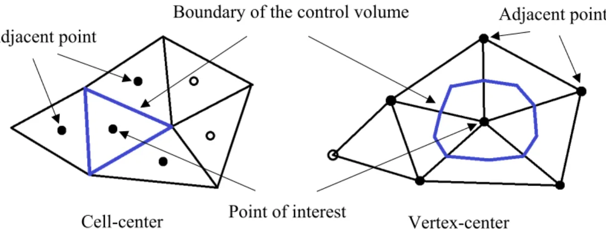
The finite volume method is also called “the control volume method”. For applying the unstructured grid, two approaches can be adopted in choosing the type of the control volume. One is to consider the cell constituted by a polyhedron as one control volume. By this method, the inspection surface is defined as the face of the cell constituted by the surrounded grid lines, on which the fluxes of physical quantities are considered. The variables are defined in the center of cells, this approach is called “the cell-center method”.

The other approach is to define the variables on vertices and build virtual inspection surfaces around the vertices to establish the control volumes, this approach is called “the vertex-center method”. The coding methods for the two approaches are called “the face- base method” and “the edge-base method”, respectively. The present software adopts the vertex-center method. Figure 3.2 shows the schematic pictures for these two considerations.

3.1.4 Convection term (小林敏雄, 2004)

For the differential scheme, various options are provided in FrontFlow/red, such as the first order upwind difference, the second order central difference and the third order TVD schemes. Here, the first order upwind difference scheme and the second order central difference scheme for the interpolation of values on the surface of a control volume (SF) are illustrated.

First order upwind difference scheme

The value on the surface of a control volume is specified using the value of the control volume in the upstream as following,

𝜙𝜙_{𝑆𝑆𝑆𝑆} = 𝜙𝜙_𝐴𝐴max (_{�𝑆𝑆⃑}^𝑆𝑆⃑^{𝑆𝑆𝑆𝑆}^{∙𝑢𝑢��⃑}^{𝑆𝑆𝑆𝑆}

𝑆𝑆𝑆𝑆∙𝑢𝑢��⃑_{𝑆𝑆𝑆𝑆}�, 0)− 𝜙𝜙_𝐵𝐵min (_{�𝑆𝑆⃑}^𝑆𝑆⃑^{𝑆𝑆𝑆𝑆}^{∙𝑢𝑢��⃑}^{𝑆𝑆𝑆𝑆}

𝑆𝑆𝑆𝑆∙𝑢𝑢��⃑_{𝑆𝑆𝑆𝑆}�, 0), (3.10) 14

(27)

where 𝜙𝜙_{𝑆𝑆𝑆𝑆} is the value on the surface that is shared by the control volume A and B, 𝜙𝜙_𝐴𝐴 and 𝜙𝜙_𝐵𝐵 are the values at control volume A and B, respectively. 𝑆𝑆⃑_{𝑆𝑆𝑆𝑆} denotes the area vector and 𝑢𝑢�⃑𝑆𝑆𝑆𝑆 denotes the velocity vector on the surface.

Second order central difference scheme

The second order central difference scheme uses the distance-weighted average value to specify the value on the surface of a control volume, which is expressed as follows,

𝜙𝜙_{𝑆𝑆𝑆𝑆} =𝑒𝑒_𝐴𝐴𝜙𝜙_𝐴𝐴+𝑒𝑒_𝐵𝐵𝜙𝜙_𝐵𝐵, (3.11)

where 𝑒𝑒_𝐴𝐴 and 𝑒𝑒_𝐵𝐵 are the weights of distance from the shared surface to the control volume A and B, respectively.

3.1.5 Gradient and diffusion term (小林敏雄, 2004)

The gradient for the control volume A is calculated using the Gauss method as follows,

∇𝜙𝜙_𝐴𝐴 = ^∑^{𝑆𝑆𝑆𝑆 𝑜𝑜𝑛𝑛}^𝑖𝑖=1 ^{𝐶𝐶𝐶𝐶𝐴𝐴}_𝛿𝛿Ω ^𝑆𝑆⃑^{𝑆𝑆𝑆𝑆𝑖𝑖}^𝜕𝜕, (3.12)

where δΩ denotes the volume of the control volume. The gradient on the surface of a control volume is calculated using the Defer-Correction-Term method proposed by Muzaferija (1994) as follows,

∇𝜙𝜙_{𝑆𝑆𝑆𝑆} =∇𝜙𝜙��_{𝑆𝑆𝑆𝑆}+_|𝑟𝑟⃑^𝑟𝑟⃑^{𝐴𝐴𝐴𝐴}

𝐴𝐴𝐴𝐴|²[(𝜙𝜙_𝐴𝐴 − 𝜙𝜙_𝐵𝐵)− 𝑟𝑟⃑_{𝐴𝐴𝐵𝐵}∙ ∇𝜙𝜙��_{𝑆𝑆𝑆𝑆}], (3.13) where ∇𝜙𝜙��_{𝑆𝑆𝑆𝑆} is the weighted average of the gradients of the control volume A and B that share the surface, 𝑟𝑟⃑_{𝐴𝐴𝐵𝐵} is the vector from vertex A to B.

3.1.6 Time integration

15

(28)

Generally, in a problem concerning the incompressible flow, no time difference of the pressure is included. Therefore, to determine the distribution of the pressure, it is necessary to combine the mass conservation equation with the other governing equations to make it always fulfilled.

Implicit methods frequently run an internal loop in updating the velocity and pressure to satisfy the continuity equation by solving the discretized equation of the velocity and pressure correction. The semi-implicit method for pressure-linked equation (SIMPLE) method is a representative example as well as its improved versions such as the SIMPLER method, the SIMPLEST method, the SIMPLEC method, the PISO method and the FIMOSE method. On the other hand, the marker and cell (MAC) method, as an explicit method, is developed and widely used for its simplicity and ease to apply on the unsteady problems. In the present software, a simplified Poisson equation is applied based on the MAC method. Also, the SMAC (simplified MAC) method is improved so that both implicit and explicit methods can be used. Also, the second-order Crank-Nicolson method, the second-order Adams-Bashforth explicit method, the third-order Adams-Moulton implicit method and the forth-order Runge-Kutta method are also available (小林敏雄, 2004).

Crank-Nicolson method (荒川忠一, 1994)

For simplification, the explanation is given by taking an example of one-dimensional unsteady heat conduction equation in a nondimensionalized form as follows:

𝜕𝜕𝜕𝜕

𝜕𝜕𝜕𝜕 =^𝜕𝜕_{𝜕𝜕𝑥𝑥}²^𝜕𝜕₂. (3.14) If the right-hand side term is computed using the averaged values of both the present (j) and next (j+1) steps, the equation could be discretized in an implicit form. When the weights of the two values are both chosen as 0.5, it is called the Crank-Nicolson implicit method, and the discretized equation is as follows

𝜕𝜕_{𝑖𝑖,𝑗𝑗+1}−𝜕𝜕_{𝑖𝑖,𝑗𝑗}

𝛿𝛿𝜕𝜕 = ¹₂(^𝜕𝜕^{𝑖𝑖+1,𝑗𝑗+1}^−2𝜕𝜕_{𝛿𝛿𝑥𝑥}^{𝑖𝑖,𝑗𝑗+1}₂ ^+𝜕𝜕^{𝑖𝑖−1,𝑗𝑗+1}+^𝜕𝜕^{𝑖𝑖+1,𝑗𝑗}^−2𝜕𝜕_{𝛿𝛿𝑥𝑥}^{𝑖𝑖,𝑗𝑗}₂^+𝜕𝜕^{𝑖𝑖−1,𝑗𝑗}), (3.15) 16

(29)

then

−𝑟𝑟𝑇𝑇_{𝑖𝑖−1,𝑖𝑖+1}+ (2 + 2𝑟𝑟)𝑇𝑇_{𝑖𝑖,𝑖𝑖+1}− 𝑟𝑟𝑇𝑇_{𝑖𝑖+1,𝑖𝑖+1} = 𝑟𝑟𝑇𝑇_{𝑖𝑖−1,𝑖𝑖}+ (2−2𝑟𝑟)𝑇𝑇_{𝑖𝑖,𝑖𝑖}+𝑟𝑟𝑇𝑇_{𝑖𝑖+1,𝑖𝑖}, (3.16)

where 𝑟𝑟= _{𝛿𝛿𝑥𝑥}^{𝛿𝛿𝜕𝜕}₂. Compared to the explicit approaches, larger time step can be set for a stable computation in the implicit method, where effective time marching can thus be achieved.

However, too large time step may cause a decrease of accuracy even though the computational stability is maintained.

MAC method (荒川忠一, 1994)

The explanation of MAC method is introduced as follows. The equations of motion and continuity for an incompressible viscous flow are shown as

𝜕𝜕𝑣𝑣�⃑

𝜕𝜕𝜕𝜕 = −∇𝑝𝑝+_{𝑅𝑅𝑅𝑅}¹ ∇²𝑣𝑣⃑ − ∇ ∙(𝑣𝑣⃑𝑣𝑣⃑), (3.17) ∇ ∙ 𝑣𝑣⃑ = 0. (3.18)

Rewrite the right-hand side of the Eq. (3.17) by a function f of 𝑣𝑣⃑ and p,

𝜕𝜕𝑣𝑣�⃑

𝜕𝜕𝜕𝜕 =𝑓𝑓(𝑣𝑣⃑,𝑝𝑝), 𝑓𝑓(𝑣𝑣⃑,𝑝𝑝) =−∇𝑝𝑝+_{𝑅𝑅𝑅𝑅}¹ ∇²𝑣𝑣⃑ − ∇ ∙(𝑣𝑣⃑𝑣𝑣⃑). (3.19)

Discretizing the equation by a forward difference,

𝑣𝑣�⃑^𝑛𝑛+1−𝑣𝑣�⃑^𝑛𝑛

∆𝜕𝜕 = 𝑓𝑓(𝑣𝑣⃑^𝑛𝑛,𝑝𝑝). (3.20)

Performing the divergence for Eq. (3.20), the following equation could be obtained,

∇∙𝑣𝑣�⃑^𝑛𝑛+1−∇∙𝑣𝑣�⃑^𝑛𝑛

∆𝜕𝜕 =∇ ∙ 𝑓𝑓(𝑣𝑣⃑^𝑛𝑛,𝑝𝑝^𝑛𝑛) =∇ ∙ 𝑓𝑓(𝑣𝑣⃑^𝑛𝑛, 0) +∇ ∙ 𝑓𝑓(0,𝑝𝑝^𝑛𝑛) =∇ ∙ 𝑓𝑓(𝑣𝑣⃑^𝑛𝑛, 0)− ∇²𝑝𝑝. (3.21)

17

(30)

To fulfill the continuity equation at time step n+1,

∇ ∙ 𝑣𝑣⃑^𝑛𝑛+1 = 0 (3.22)

is yielded, the Poisson equation for the pressure can then be obtained as

∇²𝑝𝑝 =^{∇∙𝑣𝑣�⃑}_∆𝜕𝜕^𝑛𝑛+∇ ∙ 𝑓𝑓(𝑣𝑣⃑^𝑛𝑛, 0) =^{∇∙𝑣𝑣�⃑}_∆𝜕𝜕^𝑛𝑛+_{𝑅𝑅𝑅𝑅}¹ ∇²(∇ ∙ 𝑣𝑣⃑)^𝑛𝑛− ∇ ∙(∇ ∙(𝑣𝑣⃑𝑣𝑣⃑)^𝑛𝑛). (3.23)

The procedure for the computation is concluded as follows. From the velocity at time step n, the pressure is calculated by Eq. (3.23), the velocity at time step n+1 is then calculated explicitly by Eq. (3.21) as

𝑣𝑣⃑^𝑛𝑛+1 =𝑣𝑣⃑^𝑛𝑛+∆𝑡𝑡 ∙ 𝑓𝑓(𝑣𝑣⃑^𝑛𝑛,𝑝𝑝^𝑛𝑛). (3.24)

Iterating the above operation, since the velocity at new time step is obtained, the pressure at time step n+1 can then be calculated by using the Poisson equation, the time marching approach is then established. As noted, the time marching is explicit, therefore the time step can not be set too large. Although solving the Poisson equation is popular to obtain the pressure distribution to fulfill the continuity equation, it is also known to cost much for solving it.

SMAC explicit method (小林敏雄, 2004)

As the improvement of the MAC method, in SMAC, a simplified Poisson equation is adopted and the time marching is divided into two steps to improve the accuracy. This part describes the SMAC explicit method. The momentum conservation equation is shown as follows,

𝜕𝜕^∗𝑣𝑣�⃑^∗−𝜕𝜕^𝑛𝑛𝑣𝑣�⃑^𝑛𝑛

∆𝜕𝜕 =−𝑅𝑅�⃑_{𝐵𝐵𝐶𝐶}^𝑛𝑛 − ∇𝑝𝑝^𝑛𝑛, (3.25)

𝜕𝜕^𝑛𝑛+1𝑣𝑣�⃑^𝑛𝑛+1−𝜕𝜕^∗𝑣𝑣�⃑^∗

∆𝜕𝜕 =−∇𝛿𝛿𝑝𝑝, (3.26) 18

(31)

where the superscript “*” means the intermediate value, 𝑅𝑅�⃑_{𝐵𝐵𝐶𝐶}^𝑛𝑛 means the sum of the convection term and the diffusion term, and δ𝑝𝑝 =𝑝𝑝^𝑛𝑛+1− 𝑝𝑝^𝑛𝑛 is the pressure correction.

Suppose the mass conservation is fulfilled at the new time step (n+1), the Poisson equation of the pressure correction (δ𝑝𝑝) is then obtained by performing the divergence on Eq. (3.26) as follows,

1

∆𝜕𝜕�−∇ ∙(𝜌𝜌^∗𝑣𝑣⃑^∗)�=−∇²𝛿𝛿𝑝𝑝. (3.27)

By solving this equation, the pressure correction can be calculated, and the velocity at new time step (n+1) is obtained as

𝜌𝜌^𝑛𝑛+1𝑣𝑣⃑^𝑛𝑛+1 = −∆𝑡𝑡∇𝛿𝛿𝑝𝑝+𝜌𝜌^∗𝑣𝑣⃑^∗. (3.28) The computational procedure for the explicit SMAC method is concluded as:

1. Calculate the intermediate velocity 𝑣𝑣⃑^∗ by Eq. (3.25);

2. Calculate the new pressure 𝑝𝑝^𝑛𝑛+1 =𝑝𝑝^𝑛𝑛+𝛿𝛿𝑝𝑝 by solving the Poisson equation of the pressure correction 𝛿𝛿𝑝𝑝;

3. Calculate the new velocity 𝑣𝑣⃑^𝑛𝑛+1 by Eq. (3.28);

4. Go to the next time step.

SMAC Euler implicit method (小林敏雄, 2004)

SMAC method is originally based on the explicit approach, while in the present software, an implicit approach is also available, the explanation of which is given below.

Based on the two-step procedure and replacing the explicit method in Eq. (3.25) by an implicit method, the following equations can be obtained,

𝜕𝜕^{∗𝑚𝑚+1}𝑣𝑣�⃑^{∗𝑚𝑚+1}−𝜕𝜕^𝑛𝑛𝑣𝑣�⃑^𝑛𝑛

∆𝜕𝜕 =−𝑅𝑅�⃑_{𝐵𝐵𝐶𝐶}^{∗𝑚𝑚+1}+∇𝑝𝑝^𝑚𝑚, (3.29)

𝜕𝜕^𝑚𝑚+1𝑣𝑣�⃑^𝑚𝑚+1−𝜕𝜕^{∗𝑚𝑚+1}𝑣𝑣�⃑^{∗𝑚𝑚+1}

∆𝜕𝜕 = −∇δ𝑝𝑝, (3.30) 19

(32)

where m means internal iteration number within one time step, 𝑅𝑅�⃑_{𝐵𝐵𝐶𝐶}^𝑚𝑚 is the sum of the convection term and the diffusion term, and

𝜌𝜌^{∗𝑚𝑚+1}𝑣𝑣⃑^{∗𝑚𝑚+1} =𝜌𝜌^𝑚𝑚𝑣𝑣⃑^𝑚𝑚+𝜌𝜌^′𝑣𝑣⃑^′, (3.31) δ𝑝𝑝= 𝑝𝑝^𝑚𝑚+1− 𝑝𝑝^𝑚𝑚, (3.32)

where 𝜌𝜌^′𝑣𝑣⃑^′ denotes the velocity correction in the first stage, δ𝑝𝑝 is the pressure correction.

Performing the divergence on both sides of the Eq. (3.30), ∇ ∙(𝜌𝜌^𝑚𝑚+1𝑣𝑣⃑^𝑚𝑚+1) is supposed to satisfy the continuity equation, the Poisson equation of pressure correction δ𝑝𝑝 is then obtained. Iteration within one time step is carried out until the pressure and velocity corrections are small enough, and the newest iteration value (m+1) is taken as the new value at n+1 time step.

The computational procedure of the SMAC Euler implicit method is concluded as follows:

1. Calculate the intermediate velocity by Eq. (3.29);

2. Calculate 𝑝𝑝^𝑚𝑚+1= 𝑝𝑝^𝑚𝑚+𝛿𝛿𝑝𝑝 by solving the Poisson equation of the pressure correction;

3. Calculate the new velocity 𝑣𝑣⃑^𝑚𝑚+1 by Eq. (3.30);

4. If the pressure correction is small enough and 𝑣𝑣⃑^𝑚𝑚+1 satisfies the continuity equation, the convergence is considered to be achieved.

5. If the convergence is achieved at step 4, go to the next step. Otherwise go back to step 1 and perform the next internal iteration.

3.2 Application of the direct forcing approach

Figure 3.3 shows the schematic computational procedure of FrontFlow/red (Hirose, 2013).

According to Eq. (2.8), in order to calculate the body force 𝑓𝑓_𝑖𝑖, it is necessary to obtain the desired velocity 𝑉𝑉_{𝑖𝑖𝑏𝑏}^𝑛𝑛+1 and 𝑅𝑅𝑅𝑅𝑆𝑆_𝑖𝑖. The desired velocity 𝑉𝑉_{𝑖𝑖𝑏𝑏}^𝑛𝑛+1 could be determined by setting beforehand or calculating through the feedback mechanism, while the 𝑅𝑅𝑅𝑅𝑆𝑆_𝑖𝑖 is the intermediate value during calculating 𝑢𝑢�⃑^∗, which could then be obtained by implementing a loop during the stage of solving the Navier-Stokes equations without the body force term.

Once the body force is obtained, the new velocity could be calculated by the Navier-Stokes 20

(33)

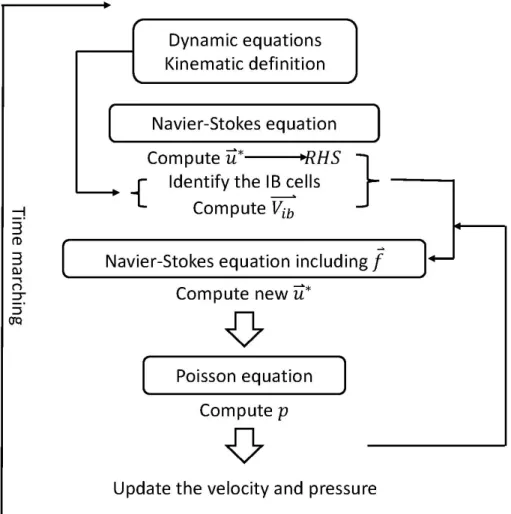
equations including the body force term. Figure 3.4 shows the schematic computational procedure including the direct forcing mechanism (Hirose, 2013). To fulfill the continuity equation (2.5), the Poisson equation is solved to update the velocity and pressure.

To carry out hydrodynamic movement in fluid, a force feedback mechanism is added into the original program. The feedback mechanism combines certain kinematic definition with the dynamic equations and uses the IB body forces as input to update the desired velocity.

The corresponding schematic computational procedure is shown in Figure 3.5. To satisfy the continuity in the immersed boundary, a rigid body system is to be adopted in the present study. The involved rigid body dynamics in the study for a single rigid body is given as follows.

Center of mass and moment of inertia

A reference point 𝑟𝑟⃑ is known as the center of mass if it satisfies the condition

∑^𝑁𝑁_𝑖𝑖=1𝑚𝑚_𝑖𝑖(𝑟𝑟��⃑ − 𝑟𝑟⃑) = 0_𝚤𝚤 . (3.33)

The moment of inertia [𝐼𝐼_𝑅𝑅] related to the center of mass is defined as

[𝐼𝐼_𝑅𝑅] =− ∑^𝑁𝑁_𝑖𝑖=1𝑚𝑚𝑖𝑖[𝑟𝑟��⃑ − 𝑟𝑟⃑]_𝚤𝚤 ², (3.34)

where [𝑟𝑟��⃑ − 𝑟𝑟⃑] = [_𝚤𝚤 0 −∆𝑟𝑟_𝑧𝑧 ∆𝑟𝑟_𝑦𝑦

∆𝑟𝑟_𝑧𝑧 0 −∆𝑟𝑟_𝑥𝑥

−∆𝑟𝑟_𝑦𝑦 ∆𝑟𝑟_𝑥𝑥 0 ].

Kinematics and dynamics

The velocity of certain point of the rigid body 𝑢𝑢��⃑ is expressed by the velocity of the center _𝚤𝚤 of mass 𝑢𝑢�⃑ and the angular velocity of the body 𝜔𝜔��⃑ as

𝑢𝑢_𝚤𝚤

��⃑=𝑢𝑢�⃑+𝜔𝜔��⃑× (𝑟𝑟��⃑ − 𝑟𝑟⃑). (3.35) _𝚤𝚤

21

(34)

The dynamic equations of force 𝐹𝐹⃑ and torque 𝑇𝑇�⃑ known as Newton’s second law of motion for a rigid body take the form as

𝐹𝐹⃑ =𝑚𝑚𝑎𝑎⃑, (3.36) 𝑇𝑇�⃑= [𝐼𝐼𝑅𝑅]𝛼𝛼⃑+𝜔𝜔��⃑× [𝐼𝐼𝑅𝑅]𝜔𝜔��⃑, (3.37)

where 𝑎𝑎⃑=𝑑𝑑𝑢𝑢�⃑ 𝑑𝑑𝑡𝑡⁄ , 𝛼𝛼⃑= 𝑑𝑑𝜔𝜔��⃑ 𝑑𝑑𝑡𝑡⁄ . When applying to the cases, some assumptions are made to simplify the computation of the dynamics. The details can be referred to Chapter 4.

An explicit scheme is adopted to perform the force feedback of dynamics. The IB force and torque at step n is taken as the input to update the movement of the rigid body using the above equations. The obtained locations and velocities of the involved vertices are then inputted into the IB subroutine to calculate the new IB force and torque at step n+1. The procedure is concluded taking the example of a single particle of radius of 𝑟𝑟₀ as follows.

1. Update the location 𝑟𝑟⃑ and orientation 𝜃𝜃⃑ of the particle by 𝑟𝑟⃑^𝑛𝑛+1 = 𝑟𝑟⃑^𝑛𝑛+𝑢𝑢�⃑^𝑛𝑛∆𝑡𝑡 and 𝜃𝜃⃑^𝑛𝑛+1 =𝜃𝜃⃑^𝑛𝑛 +𝜔𝜔��⃑^𝑛𝑛∆𝑡𝑡, respectively;

2. Calculate the acceleration of velocity (𝑎𝑎⃑^𝑛𝑛) and angular velocity (𝛼𝛼⃑^𝑛𝑛) of the particle by Eqs. (3.36) and (3.37) using 𝐹𝐹⃑^𝑛𝑛 and 𝑇𝑇�⃑^𝑛𝑛 as input;

3. Update the velocity and angular velocity of the particle by 𝑢𝑢�⃑^𝑛𝑛+1 =𝑢𝑢�⃑^𝑛𝑛+𝑎𝑎⃑^𝑛𝑛∆𝑡𝑡 and 𝜔𝜔��⃑^𝑛𝑛+1= 𝜔𝜔��⃑^𝑛𝑛+𝛼𝛼⃑^𝑛𝑛∆𝑡𝑡, respectively;

4. Update the velocity of each vertex (i) by Eq. (3.35), obtain the 𝑢𝑢�⃑_𝑖𝑖^𝑛𝑛+1;

5. Output new location 𝑟𝑟⃑^𝑛𝑛+1 and velocity 𝑢𝑢�⃑_𝑖𝑖^𝑛𝑛+1 for updating the IB force to obtain 𝐹𝐹⃑^𝑛𝑛+1 and 𝑇𝑇�⃑^𝑛𝑛+1. In case of a single particle, it is enough to determine the new boundary with only 𝑟𝑟⃑^𝑛𝑛+1 by judging whether a vertex at 𝑟𝑟⃑_𝑖𝑖 satisfies |𝑟𝑟⃑_𝑖𝑖 − 𝑟𝑟⃑|≤ 𝑟𝑟₀. For other cases, the orientation 𝜃𝜃⃑^𝑛𝑛+1 may also be needed.

The computational grid is made by the Gridgen (Gridgen) that consists of vertices and edges that connect the vertices. For the identification of the immersed region, the edge- based loop is adopted. The shape of the immersed boundary is defined using some shape function. If both the two sides of an edge fulfill the shape function, the corresponding two

22

(35)

vertices are identified as inside points. If only one side fulfills the shape function, the vertex that fulfills the function is taken as “Ghost cell” and the other one is identified as an outside point, the vertices in the vicinity of the immersed boundary could then be identified and may be used for interpolation. If both the two sides do not fulfill the shape function, the corresponding two vertices are identified as outside points. Note that in the present application, no interpolation for the velocity near the boundary is performed considering that the Reynolds numbers in the involved cases are relatively low so that the uneven boundary is thought not to bring significant influence on the computational accuracy compared to other factors, while the implementation of interpolation may cause an unstable problem.

23

(36)

Figure 3.1: The category of the cell structures.

Figure 3.2: Schematic pictures of cell-center method and vertex-center method.

Tetrahedron Pyramid

Prism Hexahedron

Boundary of the control volume

Point of interest

Adjacent point Adjacent point

Cell-center Vertex-center

24

(37)