Improvements of SAT Solving Techniques andTheir Application to the Coalition StructureGeneration Problem

Kyushu University Institutional Repository

Improvements of SAT Solving Techniques and Their Application to the Coalition Structure Generation Problem

査, 澳龍

http://hdl.handle.net/2324/1959138

出版情報：九州大学, 2018, 博士（情報科学）, 課程博士 バージョン：

権利関係：

Improvements of SAT Solving Techniques and Their Application to the Coalition

Structure Generation Problem

Zha Aolong

Improvements of SAT Solving Techniques and Their Application to the Coalition

Structure Generation Problem

Graduate School of Information Science and Electrical Engineering Department of Informatics – Fujita Laboratory

Candidate Aolong Zha

ID number 3IE15008P

Dissertation Advisors Assoc. Prof. Hiroshi Fujita Assist. Prof. Miyuki Koshimura

Co-Advisor

Prof. Ryuzo Hasegawa

A dissertation submitted in partial fulfillment of the requirements for the degree of Doctor of Philosophy in Informatics

July 2018

Assoc. Prof. Fujita Hiroshi (chairman) Prof. Yokoo Makoto

Prof. Zhao Jianjun

Improvements of SAT Solving Techniques and Their Application to the Coalition Structure Generation Problem

Ph.D. dissertation. Kyushu University

© 2018 Aolong Zha. All rights reserved

This dissertation has been typeset by L^ATEX and the Thesis class.

Version: July 22, 2018

Author’s email: [email protected]

iii

Abstract

In mathematics and computer science, there are a lot of problems that we know how to program a computer to solve “efficiently”, such as basic arithmetic, sorting a list, searching through a data structure. These problems can be solved in polynomial time, abbreviated as P. It means the number of assembly steps which are taken by summing two numbers, or sorting a list, grows manageably with the magnitude of the number or the size of the list. However, there is another class of problems for which it is quick to verify whether or not a possible solution to the problem is correct, but we do not know how to efficiently find a solution yet. This class of problems are said to be solvable in nondeterministic polynomial-time, abbreviated as N P. It is self-evident that any problem in P is automatically inN P, while to date, no one can answer the question whether or not the reverse is true. If there exists such an algorithm that could solveN P problems in polynomial time, it would have mind-blowing implications throughout most of mathematics, science and technology.

The propositional satisfiability (SAT) problem is the problem of determining if there exists an interpretation that satisfies a given propositional formula. SAT is also the first problem that was proven to beN P-complete—the “hardest” problems in N P. Various problems in artificial intelligence and computer science such as circuit/network verification, scheduling problem and constraint satisfaction problem, etc. can be reduced to SAT. Therefore, SAT problems has been emphasized for a long time and scrutinized. SAT is also interpreted in a rather broad sense. Besides plain propositional satisfiability, it includes the domains of maximum satisfiability (MaxSAT), pseudo-Boolean (PB) constraints and so on. The MaxSAT problem, an extension of SAT, is a natural combinatorial optimization problem. The essence of MaxSAT is trying to satisfy the maximum number of the constraints of a given SAT instance in the case that not all of these constraints can be satisfied. In addition, encoding PB constraints is an indispensable theory for expressing combinatorial optimization problems which can be formulated as 0–1 linear programming, and a significant effort has been devoted to the development of good SAT encoding techniques for these constraints.

The first objective of this dissertation is to speed up SAT solver. There are unit propagation and pure literal elimination (PLE) as the deduction engines of SAT solver. However, due to the data structure, detection of pure literals takes more time than detection of unit clauses, modern solvers do PLE only in preprocessing.

On the other hand, it is a feature of modern solvers to make failure learning to avoid repeating the identical contradiction when discovering inconsistency during search. Existing methods learn one conflict reason per contradiction, but generally it is possible to detect multiple conflict reasons. In this dissertation, we focus on PLE strategy, conflict detection policies, learning clause management in SAT solver, and propose two new methods to solve SAT problems more efficiently.

The enhancement of MaxSAT solver’s performance by improving the conjunctive normal form (CNF) encodings of PB constraints is the second purpose of this dissertation. The existing encodings suffer from memory-out and/or execution slow down caused by an enormous size of the encoded formula. We consider a new encoding method, which applies multiple modular arithmetic in the mixed radix base,

and we also give a tailored heuristics of the base selection for modular arithmetic. In contrast, our method achieves a compact space complexity by significantly reducing the number of auxiliary variables and clauses. Theoretically, we prove the correctness of our encoding and show that it always produces a polynomial-size CNF with respect to the number of input variables.

As the third intention in this dissertation, we practically propose one of the effec- tive applications of MaxSAT to a well-known combinatorial optimization problem, called the coalition structure generation (CSG) problem which relates to cooperative game theory and multi-agent systems. A coalition of agents can sometimes accom- plish things that individual agents cannot do or perhaps do them more efficiently.

The CSG problem is one major research topic in coalitional games—abstract models of cooperation, which involves partitioning a set of agents into coalitions to maximize social surplus, that is, the sum of the rewards of all coalitions. This dissertation handles CSG problems for partition function games, and uses partition decision trees (PDTs) as a compact representation for the utilities of possible divisions. We present and compare two methods to find optimal partitions of a set of agents for solving CSG problems. One is a branch-and-bound algorithm based on depth-first search, and the other is MaxSAT encoding and leaves the rest manipulation to MaxSAT solver. In our experiment, it is shown that the latter is probably superior to the former when the PDT rules are negative. Furthermore, the latter’s standard deviation of runtime is empirically less than the former’s.

The established contributions of this dissertation are summarized as follows.

1. Speeding up modern SAT solvers by two original efficient implementations 2. Enhancing MaxSAT solver by improving CNF encoding of PB constraints 3. Demonstrating the efficiency of our MaxSAT solver through solving CSG

problems

v

Acknowledgments

First of all, I would like to express my sincere gratitude to my dissertation advisors, Miyuki Koshimura and Hiroshi Fujita for their valuable suggestions.

I am deeply indebted to Japan Student Services Organization and Kyushu Uni- versity, for giving me financial support which was indispensable to my living.

Besides, I am grateful to Naoki Uemura, Toshitaka Arimura, Xiaojuan Liao, Emiko Masunaga and all other members of Fujita Laboratory, for continuously encourage me, and giving various support to my research.

I would also like to acknowledge my collaborators, Kazuki Nomoto, Yuko Sakurai, Suguru Ueda and Makoto Yokoo for providing me with an opportunity to work on a cooperative research.

My special appreciations go to professor Jianjun Zhao for his precious comments.

Last, but not least, I would like to thank my family: Jinping, Shanjun and Qingzhou for everything; Yuhua for her devoted support; Jiajia and Yangyang for

filling my life with pleasure.

vii

Contents

1 Introduction 1

1.1 Logical System . . . 1

1.2 Propositional Logic . . . 2

1.2.1 Boolean algebra . . . 2

1.2.2 Circuit satisfiability problem . . . 3

1.2.3 Conjunctive normal form . . . 4

1.2.4 Propositional satisfiability problem . . . 8

1.3 Intractability . . . 9

1.3.1 Asymptotic bounds. . . 9

1.3.2 Complexity issues . . . 10

1.3.3 Reductions . . . 12

1.4 Organization . . . 14

2 SAT Algorithms 15 2.1 The DPLL Algorithm . . . 16

2.1.1 Unit propagation . . . 17

2.1.2 Chronological backtracking . . . 17

2.2 Search and Inference . . . 19

2.2.1 Implication graph . . . 19

2.2.2 Deriving a conflict-driven clause . . . 20

2.2.3 Asserting clauses . . . 20

2.2.4 Backtracking Scheme. . . 21

2.3 Organization of CDCL Solver . . . 22

3 Efficient Implementations 25 3.1 Pure Literal Elimination . . . 26

3.1.1 Priorities of variable assignment . . . 26

3.1.2 Pure literal detection. . . 27

3.1.3 Dummy decision assignment. . . 28

3.1.4 GlucosePLEin SAT competition 2016 . . . 28

3.2 Clauses Learning and Deletion . . . 29

3.2.1 Watched literal data structure . . . 29

3.2.2 Breadth-extended approach . . . 31

3.2.3 Clause deletion strategies and policies . . . 32

3.2.4 GluHack in SAT competition 2018 . . . 33

4 Pseudo-Boolean Constraint Encoding for MaxSAT 35

4.1 Maximum Satisfiability Problem . . . 35

4.2 QMaxSATsolver . . . 36

4.3 Totalizer Based Encoding . . . 39

4.3.1 Totalizer. . . 39

4.3.2 Weighted totalizer . . . 43

4.4 N-level Modulo Totalizer Encoding . . . 45

4.4.1 Single-level modulo. . . 45

4.4.2 Multi-level modulo . . . 49

4.4.3 Selecting suitable mixed radix base . . . 52

4.5 Implementation and Evaluation . . . 54

4.6 Related Works . . . 58

5 Practical Problems 61 5.1 Related Works . . . 62

5.2 Preliminaries . . . 62

5.3 Partition Decision Trees . . . 64

5.4 Branch-and-Bound Algorithm . . . 65

5.4.1 Naive algorithm for positive rules . . . 66

5.4.2 Algorithm using modified PDTs. . . 66

5.5 MaxSAT Encoding . . . 68

5.6 Experimental Results. . . 69

6 Conclusions and Future Work 75

ix

List of Tables

1.1 Cross-reference table between syntax and semantics . . . 1 1.2 The running times (rounded up) of different algorithms on inputs

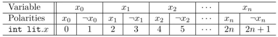
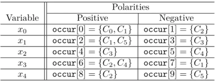
of increasing size, for a processor performing a million high-level instructions per second. In cases where the running time exceeds 10²⁵ years, we simply record it by an∞ symbol. . . 10 3.1 The correspondence of indexes between literal and variable. . . 26 3.2 The initialization of the array occurfor the instance in Formula 3.1. 28 4.1 Encoding PB constraint 147x₁+ 540x₂+ 1365x₃ <2018 by 4-level

MTO with vectors of moduli Λ₁=h5,5,5,5iand Λ₂=h3,7,5,6i . . 53 4.2 Average runtimes and number of instances solved . . . 56 5.1 {MPDT, MaxSAT} for {uniform, NDCS} distribution with 100 agents 71 5.2 {MPDT, MaxSAT} for {uniform, NDCS} distribution with 200 agents 72

xi

List of Figures

1.1 A circuit with three inputs, two additional sources that have assigned truth values, and one output. . . 4 1.2 A mind map drawing the range of SAT-based techniques in different

development directions . . . 9 2.1 A search tree of enumerating all truth assignments over Boolean

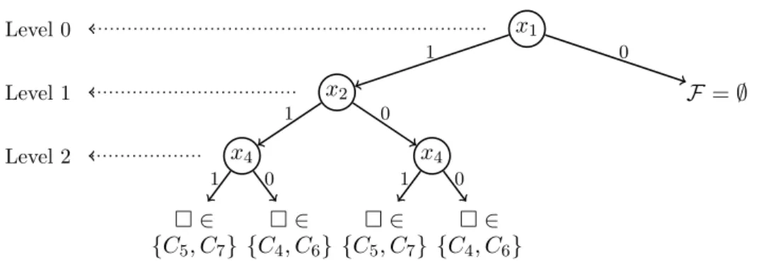
variablesx₁,x₂ and x₃ in decision variable order−−−−→x₁x₂x₃ which cor- responds the decision levels from top to bottom in the leftmost of figure. . . 16 2.2 A termination tree. Assignments shown next to nodes are derived

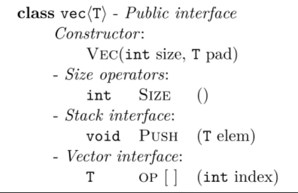
using UP. . . 19 2.3 Two cuts in an implication graph, and an example of a UIP. . . 20 3.1 A basic abstract data type vechTi used throughout the code. . . 25 3.2 A demonstration of the watched literal data structure for clause

(x₁∨ ¬x₂∨x₃∨x₄∨ ¬x₅). After initialization (A), two watched literal references (pointersw₁ and w₂) keep updating (fromB toD), until the clause is declared unit (E). Then a conflict occurs via UP (F), and no reference need to move (undo) during backtracking (G). . . . 30 3.3 An abridged implication graph illustrating several conflicts occurring

in the same decision level. . . 32 3.4 A glimpse of the watch list (only corresponding clauses from C₁ to

C₉) on the brink of backtracking in Example 9, also illustrated in Figure 3.3. C₁ is the sequence of assignment which is duplicated from Fin Figure 3.2. The conflicts 1 and 2 (resp. conflicts 3 and 4) belong to the conflict pattern 1 (resp. pattern 2). . . 33 4.1 TO encoding: (a) Overview over binary tree of TO adders showing

connection of input and output between each recursion. (b) Detailed adder for two input vectors of Boolean variables. . . 42 4.2 Comparison of cumulative #Instances solved in generated #variables

and #clauses . . . 57 4.3 Comparison of cumulative #Instances solved within runtime. . . 58 4.4 Comparison of runtimes of each instance solved with n-level MTO

and MaxHS . . . 58 5.1 PDTs of coalitional game given in Example 19 . . . 65

5.2 Modified PDTs of coalitional game given in Example 19 . . . 67

5.3 A search tree for the modified PDTs in Figure 5.2 . . . 67

5.4 Uniform vs. NDCS in MPDT . . . 73

5.5 Uniform vs. NDCS in MaxSAT . . . 73

xiii

List of Algorithms

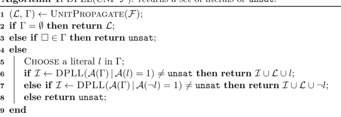
1 DPLL(CNFF): returns a set of literals orunsat. . . 18

2 CDCL(CNF F): returns satorunsat. . . 22

3 The occurrence of each literal in corresponding clause(s). . . 27

4 Pure literal detection algorithm in solving process . . . 29

5 QMaxSAT(F_w^b): returnkopt . . . 38

6 TO(h(w₁, b₁). . .(w_m, b_m)i): return (Z_sum,Φ) . . . 41

7 WTO(h(w₁, b₁). . .(w_m, b_m)i): return (Z_sum,Φ). . . 44

8 1LvMTO(h(w₁, b₁). . .(wm, bm)i, p): return (U_z|_pL_z,Φ) . . . 48

9 nLvMTO(h(w₁, b₁). . .(w_m, b_m)i,Λ) : return (D_zⁿ⁺¹|_λn. . .|_λ1D_z¹,Φ) . . 51

10 BaseSelection(h(w₁, b₁). . .(w_m, b_m)i, κ): return Λ . . . 55

1

Chapter 1

Introduction

1.1 Logical System

Among the important properties that logical systems can have:

• Validity, which means that an argument never allows a false conclusion (specif- ically, inference) from true premises.

• Consistency, which means that no theorem of the system contradicts another.

• Completeness, which means that if an argument is true, it can be proven to be a theorem of the system.

These properties are interdefinable if we make use of negation (in symbol ¬): the argument from φ₁, . . . , φn to ψ is valid if and only if the set {φ₁, . . . , φn,¬ψ} is inconsistent, which can be understood as if it would be impossible for them all to be true. Validity and consistency are really two ways of looking at the same thing and each may be described in terms of syntax or semantics in Table1.1.

Syntax, giving rise to proof theory, is restricted to definitions that refer to the syntactic form (grammatical structure) of the sentences in question. Proofs are derived with respect to anaxiom system which is defined syntactically as consisting of a set of axioms and inference rules that sanction proof steps with specified grammatical forms. In contrast, semantics, giving rise tomodel theory, studies the way sentences relate to “the world”. A sentence is said to be true if it “corresponds to the world”. The concept ofalgebraic structureis used to make precise the meaning of

“corresponds to the world”. We will speak of formulae instead of sentences to allow Table 1.1. Cross-reference table between syntax and semantics

Logic Syntax Sematics

Validity Derivability Validity

Consistency Consistency Satisfiability

Theory Proof theory Model theory

System Axiom system Formula system

Structure Grammatical structure Algebraic structure Consequence Syntactic entailment|− Semantic entailment|=

for the possibility that a sentence includes free variables. The customary notation is to use A |=φto sayφ is true in the structureA(premise). Intuitively, an argument is valid if whenever the premises are true, so is the conclusion. Satisfiability is the semantic version of consistency. A set of formulae is said to besatisfiable if there is some structure in which all its component formulae are true: that is,{φ₁, . . . , φ_n}is satisfiable if and only if, for some A,A |=φ₁ and. . . andA |=φn. It follows from the definitions that validity and satisfiability are mutually definable: φ₁, . . . , φn|=ψ if and only if {φ₁, . . . , φ_n,¬ψ} isunsatisfiable.

There is a further pair of basic logical ideas closely related to satisfiability:

necessity andpossibility. Semantically, a sentence is said to be necessary (necessarily true) if it satisfies all models, and possible (possibly true) if it satisfies at least one model. If we understand a model (possible world) to be a structure, possibility turns out to be just another name for satisfiability. In logic, the technical name for a necessary formula istautology(>): φis defined to be alogical truth(in symbols,|=φ) if and only if, for all A,A |=φ. There is also a syntactic version of a logical truth, namely a theorem-in-an-axiom-system. We say φis a theorem of the system if and only if φis derivable from the axioms alone. In a complete system, theorem-hood and logical truth coincide: |−φiff|=φ. Therefore, in logical truth and theorem-hood we encounter yet another pair of syntactic and semantic concepts that, although they have quite different sorts of definitions, nevertheless coincide exactly. Moreover, a formula is necessary if it is not possibly not true. In other words, |=φif and only if it is not the case that φis unsatisfiable. Ergo, satisfiability, theorem-hood, logical truths and necessities are mutually “characterizable”.

This review shows how closely related satisfiability is to the central concepts of logic. Indeed, relative to a complete axiom system, satisfiability may be used to define, and may be defined by, the other basic concepts of the field—validity, consistency, completeness, logical truth, tautology, and theorem-hood.

1.2 Propositional Logic

Propositional logic is a logical system that is intimately connected to Boolean algebra.

Many syntactic concepts of Boolean algebra carry over to propositional logic with only minor changes in notation and terminology, while the semantics of propositional logic are defined via Boolean algebras in a way that the tautologies (theorems) of propositional logic correspond to equational theorems of Boolean algebra.

1.2.1 Boolean algebra

George Boole (1815-1864) advanced the state of logic considerably with the introduc- tion of the algebra structure that bears his name: a structure A=hB,∨,∧,¬,0,1i is a Boolean algebra if and only if ∨ and∧ are binary operations and ¬is a unary operation on domain B under whichB is closed, 1,0∈B, and satisfies the following rules and laws:

Commutation

(x∨y=y∨x

x∧y=y∧x Identity

(x∨0 =x x∧1 =x

1.2 Propositional Logic 3

Absorption

(x∨(x∧y) =x

x∧(x∨y) =x Annihilation

(x∨1 = 1 x∧0 = 0 Association

(x∨(y∨z) = (x∨y)∨z

x∧(y∧z) = (x∧y)∧z Idempotence

(x∨x=x x∧x=x Distribution

(x∨(y∧z) = (x∨y)∧(x∨z)

x∧(y∨z) = (x∧y)∨(x∧z) Complementation

(x∨ ¬x= 1 x∧ ¬x= 0 De Morgan

(¬x∨ ¬y=¬(x∧y)

¬x∧ ¬y=¬(x∨y) Double negation ¬(¬x) =x Boolean algebra was introduced in Boole’s first book The Mathematical Analysis of Logic, and set forth more fully in his An Investigation of the Laws of Thought.

His main innovation was to develop an algebra-like notation for the elementary properties of sets. He was one of the first to employ a symbolic language. Boole was not interested in axiom systems, but in the theory of inference. In his system it could be shown that the argument fromφ₁, . . . , φntoψis valid (i.e. φ₁, . . . , φn|=ψ) by deriving the equationψ from equationsφ₁, . . . , φ_n by applying rules of inference, which were essentially cases of algebraic substitution.

Syntactically, every Boolean term corresponds to a propositional formula of propositional logic. The semantics of propositional logic rely on truth assignments.

The essential idea of a truth assignment is that the propositional variables are mapped to elements of a fixed Boolean algebra, and then the truth value of a propositional formula using these letters is the element of the Boolean algebra that is obtained by computing the value of the Boolean term corresponding to the formula.

A tautology is a propositional formula that is assigned truth value 1 by every truth assignment of its propositional variables to an arbitrary Boolean algebra.

These semantics permit a translation between tautologies of propositional logic and equational theorems of Boolean algebra. Every tautology φ of propositional logic can be expressed as the Boolean equation φ= 1, which will be a theorem of Boolean algebra. Conversely every theoremφ=ψ of Boolean algebra corresponds to the tautologies (φ∧ψ)∨(¬φ∧ ¬ψ) and (¬φ∨ψ)∧(¬ψ∨φ). If the operator →, named “implies”, is in the language these last tautologies can also be written as (φ→ψ)∧(ψ→φ), or as two separate theoremsφ→ψ and ψ→φ.

1.2.2 Circuit satisfiability problem

There is a great idea about modern computing that is to let a combinatorial logic circuit, e.g., acentral processing unit (CPU), calculates complex problems of the real world. To specify circuit satisfiability (CircuitSAT) problem, we need to make precise what we mean by acircuit. Consider the basic operators of Boolean algebra:

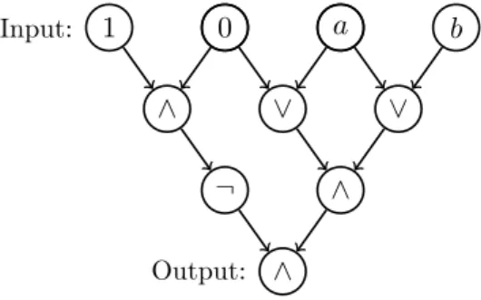
∨,∧, and ¬. Our definition of a circuit, referring to [44], is designed to represent a digital electronic circuit built out of gates that implement these operators. Thus we define a circuitK to be a labeled, directed acyclic graph such as the one shown in the example of Figure1.1.

• Thesources inK (the nodes with no incoming edges) are labeled either with

one of the constants 0 or 1, or with the name of a distinct Boolean variable.

The nodes of the latter type will be referred to as the inputs to the circuit.

• Every other node is labeled with one of the Boolean operators∨,∧, or¬; nodes labeled with∨ or∧will have two incoming edges, and nodes labeled with ¬ will have one incoming edge.

• There is a single node with no outgoing edges, and it will represent the output:

the result that is computed by the circuit.

A circuit computes a function of its inputs in the following natural way. We imagine the edges as “wires” that carry the 0/1 signal value at the nodes they emanate from.

Each node other than the sources will take the values on its incoming edge(s) and apply the Boolean operator that labels it. The result of this ∨,∧, or¬ operation will be passed along the edge(s) leaving this node. The overall value computed by the circuit will be the value computed at the output node.

∧

¬

∧

1 0

∧

∨ ∨

a b

Output:

Input:

Figure 1.1. A circuit with three inputs, two additional sources that have assigned truth values, and one output.

For example, consider the circuit K in Figure1.1. The leftmost two sources are preassigned the values 1 and 0, and the next three sources constitute the inputs. If the input Boolean variable ais assigned to value 1, then we get values 0, 1, 1 for the gates in the second row, values 1, 1 for the gates in the third row, and the value 1 for the output. Symbolically, this circuit K can be represented as a propositional logic formula:

F_K =¬(1∧0)∧((0∨a)∧(a∨b)) =a

Now, the CircuitSAT is the following decision problem. We are given a circuitK (or its propositional logic formulaF_K) as an input, and we need to decide whether there is an assignment of values to the inputs that causes the output to take the value 1. (If so, we will say that the given circuit is satisfiable, and a satisfying assignment is one that results in an output of 1.) In our example, we have just seen—via the assignment a= 1—that the circuit K in Figure 1.1is satisfiable.

1.2.3 Conjunctive normal form

Propositional logic formulae can be transformed (encoded) to conjunctive normal form (CNF): a conjunction ofclauses ^V_iC_i, each clause C_i being a disjunction of literals ^W_jlj, and each literallj being either a Boolean variable x or its negation¬x.

In this dissertation, a CNF formula (resp. a clause) can also be regarded as a set of

1.2 Propositional Logic 5

conjunctive clauses (resp. a set of disjunctive literals). CNF has the advantage of being a very simple form, leading to easy algorithm implementation and a common file format. Unfortunately, there are several ways of encoding most combinatorial problems, and few guidelines on how to choose among them, yet the choice of encoding can be as important as the choice of search algorithm. Different encodings may have different advantages and disadvantages such as space complexity or solution density, and what is an advantage for one SAT solver might be a disadvantage for another. In short, CNF encoding is an art and we must often proceed by intuition and experimentation.

Transformation by Boolean algebra

A propositional logic formula can be transformed to a logically equivalent CNF formula by using the rules and laws of Boolean algebra.

Example 1. Consider the propositional formula (a→(c∧d))∨(b→(c∧e)).

The implications can be decomposed:

((a→c)∧(a→d))∨((b→c)∧(b→e)).

The conjunctions and disjunctions can be rearranged:

((a→c)∨(b→c))∧((a→c)∨(b→e))∧

((a→d)∨(b→c))∧((a→d)∨(b→e))

The implications can be rewritten as disjunctions, and duplicated literals removed:

(¬a∨ ¬b∨c)∧(¬a∨ ¬b∨c∨e)∧(¬a∨ ¬b∨c∨d)∧(¬a∨ ¬b∨d∨e) Finally, subsumed clauses can be removed, leaving the conjunction

(¬a∨ ¬b∨c)∧(¬a∨ ¬b∨d∨e)

This example reduces to a compact CNF formula, but in general this method yields exponentially large formulae.

Transformation by Tseitin encoding

Conversion to CNF is more usually achieved using the well-known Tseitin encodings [70], which generate a linear number of clauses at the cost of introducing a linear number of new Boolean variables, and generate anequisatisfiable formula (satisfiable if and only if the original formula is satisfiable). Tseitin encodings work by adding fresh auxiliary variables to the CNF formula, one for every non-clausal subformula of the original formula, along with clauses to capture the relationships between these auxiliary variables and the subformulae.

Example 2. On the Example1 the Tseitin encoding would introduce an auxiliary variablex with definition

x↔(c∨d)

to represent subformula (c∨d). This definition can be reduced to clausal form:

(¬x∨c)∧(¬x∨d)∧(¬c∨ ¬d∨x) Similarly it would introduce another definition

y ↔(c∨e) which reduces to clauses

(¬y∨c)∧(¬y∨e)∧(¬c∨ ¬e∨y) Applying these definitions the original formula is reduced to

(¬a∨x)∨(¬b∨y) which can be finally rewritten as a clausal form

(¬a∨x∨ ¬b∨y)

Transformation from CNF to 3-CNF

3-CNF formulae, also referred to as instances of 3-SAT problem have exactly three literals in each clause. These problems are interesting in their own right, and random 3-CNF problems have been extensively studied. A CNF formula can be transformed to a 3-CNF formula as follows. For a clause ci = (l₁∨. . .∨l_k) there are four cases:

k =1 Create two new variablesbi,1, bi,2 and replace ci by the clauses (l₁∨bi,1∨ b_i,2),(l₁∨ ¬b_i,1∨b_i,2),(l₁∨b_i,1∨ ¬b_i,2) and (l₁∨ ¬b_i,1∨ ¬b_i,2).

k =2 Create one new variableb_i,1 and replacec_i by the clauses (l₁∨l₂∨b_i,1) and (l₁∨l₂∨ ¬b_i,1).

k =3 Leave clauseci unchanged.

k >3 Create new variables bi,1, bi,2, . . . , bi,k−3 and replace ci by the clauses (l₁∨ l₂∨b_i,1),(¬b_i,1∨l₃∨b_i,2),(¬b_i,2∨l₄∨b_i,3), . . . , (¬b_i,k−3∨lk−1∨l_k).

This transformation does not seen to have many practical applications, but it may be useful for generating 3-CNF benchmarks, or as a preprocessor for a specialized algorithm that only accepts instances of 3-SAT problem.

1.2 Propositional Logic 7

Extensional constraints in CNF

One way of modelling a problem, e.g., n-Queens, Sudoku, etc., as SAT is first to model it as a constraint satisfaction problem (CSP), then to apply a standard encoding from CSP to SAT.

8

0ZqZ0Z0Z

7

Z0Z0l0Z0

6

0l0Z0Z0Z

5

Z0Z0Z0Zq

4

qZ0Z0Z0Z

3

Z0Z0Z0l0

2

0Z0l0Z0Z

1

Z0Z0ZqZ0

a b c d e f g h

2 6

1 7

3 1 6

6 5 8 3

9 2 6 1 7

5 4 8 6

8 4 3

4 8

9 4

A finite-domain CSP has variables v₁. . . vn each with a finite domain, and constraints prescribing prohibited combinations of values. The problem is to find an assignment of values to all variables such that no constraint is violated. The most natural and widely-used encoding from CSP to SAT isdirect encoding. A SAT variable (i.e., Boolean variable)x_v,i, is defined as true if and only if the CSP variable v has the domain valueiassigned to it. The direct encoding consists of three sets of clauses. Each CSP variable must take at least one domain value, expressed by at-least-one clauses:

_

i

x_v,i

No CSP variable can take more than one domain value, expressed byat-most-one clauses:

¬x_v,i∨ ¬x_v,j Conflicts are enumerated byconflict clauses:

¬x_v,i∨ ¬x_w,j

Example 3 (Graph coloring problem). Given two adjacent vertices v andw and three available colors{0,1,2}, each vertex must take exactly one color, but because they are adjacent they cannot take the same color. The direct encoding of the problem contains at-least-one clauses

(xv,0∨xv,1∨xv,2) (xw,0∨xw,1∨xw,2) at-most-one clauses

(¬x_v,0∨ ¬x_v,1) (¬x_v,0∨ ¬x_v,2) (¬x_v,1∨ ¬x_v,2) (¬x_w,0∨ ¬x_w,1) (¬x_w,0∨ ¬x_w,2) (¬x_w,1∨ ¬x_w,2)

and conflict clauses

(¬x_v,0∨ ¬x_w,0) (¬x_v,1∨ ¬x_w,1) (¬x_v,2∨ ¬x_w,2) This problem has six solutions:

[v= 0, w= 1] [v= 0, w= 2] [v= 1, w= 0]

[v= 1, w= 2] [v= 2, w= 0] [v= 2, w= 1]

1.2.4 Propositional satisfiability problem

Definition 1 (Propositional satisfiability problem). Given a CNF formulaF over a finite set of Boolean variables X ={x₁, . . . , x_n}, the propositional satisfiability (SAT) problem is the decision problem of determining if there exists a truth assign- ment that satisfies F = 1. A (partial) truth assignment is function A:X7→ {0,1}, whereX ⊂X. This function can be extended to variables inX \X, literals, clauses and CNF formulae, resulting in a function from formulae to formulae as follows:

• For variables, xi ∈/X,A(x_i) =xi.

• For literals, A(¬x_i) = 1− A(x_i), ifx_i∈X; otherwise,A(l) =l.

• For clauses, A(l₁∨. . .∨lr) = A(l₁)∨. . .∨ A(l_r), and A() = 0, simplified considering 1∨C = 1 and 0∨C=C.

• For CNF formulae, A(C₁∧. . .∧C_m) =A(C₁)∧. . .∧ A(C_m) and A(∅) = 1, simplified considering 1∧ F =F and 0∧ F = 0.

A total truth assignment is truth assignment A with domain X. Note that, di- acritically, we denote the empty clause and the empty CNF formula as and ∅ respectively. For any CNF formula, A(F) may be 0, 1, or a partial instantiation of F, whereas for total truth assignments,A(F) is either 0 or 1. Truth assignmentA satisfies a literal, clause, or a CNF formula if it assigns 1 to it, andfalsifies it if it assigns 0. Thus a CNF formula is satisfiable if there exists a truth assignment that satisfies it. Otherwise, it is unsatisfiable.

There is a special case of SAT that will turn out to be equivalently difficult and is somewhat easier to think about; this is the case in which all clauses contain exactly three literals. We call this problem 3-SAT. On the other hand, SAT is special case of CircuitSAT as a CNF formula can be represented as a circuit.

SAT and 3-SAT are really fundamental combinatorial search problems; they contain the basic ingredients of a hard computational problem in very “bare-bones”

fashion. We have to make nindependent decisions (the assignments for eachxi) so as to satisfy a set of constraints. There are several ways to satisfy each constraint in isolation, but we have to arrange our decisions so that all constraints are satisfied simultaneously.

SAT is interpreted in a rather broad sense. Besides plain propositional satisfiabil- ity, it includes the domains of maximum satisfiability (MaxSAT) and pseudo-Boolean (PB) constraints, quantified Boolean formulae (QBF), satisfiability modulo theories (SMT), constraints programming (CSP) techniques, etc., for word-level problems

1.3 Intractability 9

SAT

CSP

RCF SMT QBF

Finite Model Finding

ASP

All- SAT

BDD #SAT

Max- SAT

PBS

PBO

MIP

Automated Theorem Proving

Computer algebra

Linear Arithmetic

Mathematical optimization

Enumeration

Predicatelogic

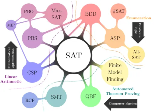
Figure 1.2. A mind map drawing the range of SAT-based techniques in different develop- ment directions

and their propositional encodings. Figure 1.2is a mind map of paradigmatic SAT- based techniques which depicts such extended and related fields of SAT in different development directions (corresponding various problem classes).

1.3 Intractability

When people first began analyzing discrete algorithms mathematically, a consensus began to emerge on how to quantify the notion of a “reasonable” running time. The asymptotic viewpoint is inherent to computational complexity theory. In virtue of polynomials typify “slowly growing” functions, we’d like an efficient algorithm to have a better scaling property: when the input size increases by a factor, its running time should be only bounded by a power of this factor.

1.3.1 Asymptotic bounds

Our discussion of computational tractability has turned out to be intrinsically based on our ability to express the notion that an algorithm’s worst-case running time on inputs of sizen grows at a rate that is at most proportional to some functionf(n).

Then f(n) becomes a bound on the running time of the algorithm.

Definition 2 (Asymptotic notations). Letf(n) and g(n) be two functions. If there exist constants (independent ofn) , csuch that 0< < c, and n₀≥0 so that for all n≥n₀ (i.e., for sufficiently largen), we have different asymptotic notations for corresponding conditions as follows:

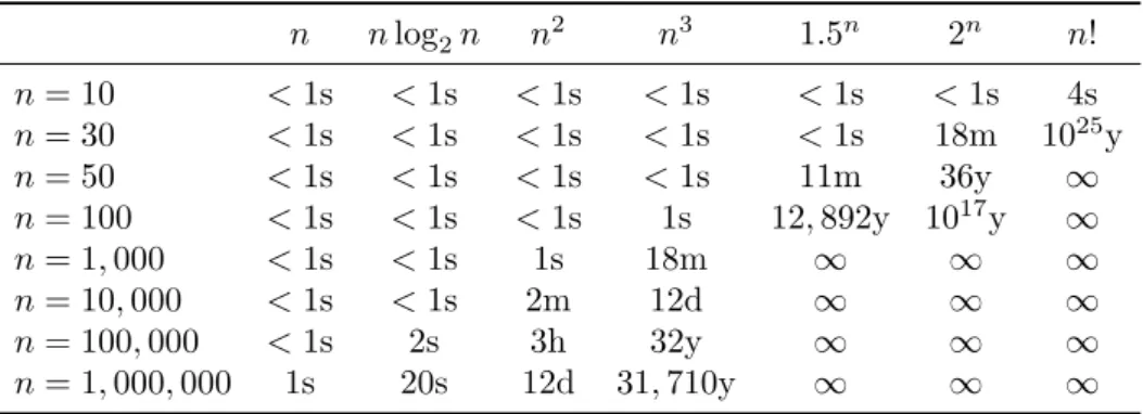
Table 1.2. The running times (rounded up) of different algorithms on inputs of increasing size, for a processor performing a million high-level instructions per second. In cases where the running time exceeds 10²⁵ years, we simply record it by an ∞symbol.

n nlog₂n n² n³ 1.5ⁿ 2ⁿ n!

n= 10 <1s <1s <1s <1s <1s <1s 4s

n= 30 <1s <1s <1s <1s <1s 18m 10²⁵y

n= 50 <1s <1s <1s <1s 11m 36y ∞

n= 100 <1s <1s <1s 1s 12,892y 10¹⁷y ∞

n= 1,000 <1s <1s 1s 18m ∞ ∞ ∞

n= 10,000 <1s <1s 2m 12d ∞ ∞ ∞

n= 100,000 <1s 2s 3h 32y ∞ ∞ ∞

n= 1,000,000 1s 20s 12d 31,710y ∞ ∞ ∞

O If f(n)≤c·g(n), then we say thatf is asymptotic upper-bounded by g, and denoted it as f(n) =O(g(n));

Ω If·g(n)≤f(n), then we say thatf is asymptotic lower-bounded byg, denoted asf(n) = Ω(g(n));

Θ If ·g(n)≤f(n)≤c·g(n), then we say thatf is asymptotic tight-bounded by g, denoted as f(n) = Θ(g(n));

Definition 3 (Primitive computational step). In Touring machine, each primitive computational step corresponds to a single instruction of machine language on a standard processor. In particular, one primitive computational step is in O(1).

Definition 4 (Polynomial-time algorithm). There are constants c >0 and d >0 so that on every input instances of size n for an algorithm, if its running time is bounded by cn^d primitive computational steps, i.e., the algorithm is O(n^d), then it is a polynomial-time algorithm.

Problems for which polynomial-time algorithms exist almost invariably turn out to have algorithms with running times proportional to very moderately growing polynomials liken, nlog₂n, n²,orn³. Conversely, problems for which no polynomial- time algorithm is known tend to be very difficult in practice. For example, search spaces for combinatorial problems tend to grow exponentially in the size nof the instance¹; if the instance size increases by one, the number of possibilities increases multiplicatively. Suppose that we have a processor that executes a million high- level instructions per second, and we have algorithms with running-time bounds of n, nlog₂n, n², n³,1.5ⁿ,2ⁿ,and n!. In Table1.2, we show the running times of these algorithms (in seconds, minutes, days, or years) for inputs of size n= 10, 30, 50, 100, 1,000, 10,000, 100,000 and 1,000,000.

1.3.2 Complexity issues

Much of complexity theory deals with decision problems. A decision problem is any arbitrary yes/no question on an infinite set of instances. Decision problems fall into

1 An instance of a problem is considered as an input of an algorithm that can solve it.

1.3 Intractability 11

sets of comparable complexity, called complexity classes. P andN P are the most well-known complexity classes, named as an acronym for “polynomial-time” and

“nondeterministic polynomial-time”, respectively.

Definition 5 (Complexity class P). P is the set of decision problems each of whose containing instances can be solved (yes/no) by a polynomial-time algorithm.

Distinctively, those of yes-instance consist inP_yes, those of no-instance consist in P_no, and we always haveP =P_yes∪ P_no.

Example 4 (Is-Primeproblem). Given an integern(n≥2), Is-Primeproblem asks whethernis a prime number or not. There exists algorithm AKS(n) [4] that returns answer yes/no in O(log⁶₂n). Notice that no matter instance (input)n is either a prime number (inP_yes) or a composite number (inP_no),Is-Prime problem belongs to P.

Definition 6 (Complexity class N P). N P is the set of decision problems each of whose including instances must have at least one yes-solution, and there exists a yes-solution can be verified by a polynomial-time algorithm (verifier).

Corollary 1. P_yes⊆ N P

Proof. LetXbe any problem inP_yes. By Definition5, there exists a polynomial-time algorithmA that solves (returnsyes) all instances ofX. We have a polynomial-time verifier B(n, s) simply returns the valueA(n), where nis any instance ofX andsis one of the yes-solution ofn.

While the Definition 5 is symmetric², the the Definition 6 is fundamentally asymmetric. Having efficient certificates that a given object has property C, does not automatically entail having nice certificates that a given object doesn’t have it. An input n is a yes-instance if and only if there exists a solution s so that B(n, s) =yes. Negating this statement, we see that an input nis a no-instance if and only if for alls, it is the non-solution case that B(n, s) =no.

Definition 7 (Complexity class co-N P). co-N P is the set of decision problems whose complements are in N P.

Example 5 (Is-Composite problem). Given an integer n(n≥2), Is-Composite problem asks whethernis a composite number or not. If there exists ayes-solution swhich can be interpreted as n, then it can be verify by algorithm Prod(n, s) in O(1). Notice that Is-Compositeproblem belongs to N P only for whose instances (inputs) exactly are composite numbers and there exists such their yes-solutions.

Alternatively, for those inputs of prime number,Is-Compositeproblem is in co-N P by Corollary1 and Definition7, becauseIs-Prime problem (this case is inP_yes) is the complement of Is-Compositeproblem.

Corollary 2. P_no⊆ co-N P

2 Having an efficient algorithm to determine if an object has a propertyCis equivalent to having an efficient algorithm for the complementary setC.

There is a famous anecdote of a lecture by F. N. Cole, entitled “On the Fac- torization of Large Numbers”, at the 1903 American Mathematical Society (AMS) meeting. Without uttering a word, he went to the chalkboard, wrote

2⁶⁷−1 = 147573952589676412927 = 193707721×761838257287

and proceeded to perform the long multiplication of the integers on the right hand side to derive the integer on the left: Mersene’s 67-th number (which was conjectured to be prime). No one in the audience had any questions. Cole demonstrated that the number 2⁶⁷−1 is composite, and the proof is simply a nontrivial factor of it. The fact that it was extremely hard for Cole to find these factors (he said it took him

“three years of Sundays”) did not affect in any way that demonstration. It is taken for granted that the written proof is succinct and efficiently verifiable, regardless how long it took to discover, which is the features we want to extract from this motivating episode.

1.3.3 Reductions

Theoretical computer scientists explore the space of computationally hard problems, eventually arriving at a mathematical characterization of a large class of them. The basic technique in this exploration is to compare the relative difficulty of different problems; we want to formally express statements like, “Problem Y is at least as hard as problemX.”

Definition 8 (Polynomial-time Turing reduction). Problem X is polynomial-time Turing reducible to problemY if (1) arbitrary instances of X can be solved using a polynomial number of calls to a subroutine that solves arbitrary instances of Y, and (2) polynomial time outside of those subroutine calls. We call this reduction a polynomial-time Turing reduction, a.k.a, Cook reduction, and denote it as X≤_p Y.

X≤_p Y can be understood as “Y is at least as hard asX”, since supposeX≤_p Y, (1) if Y can be solved in polynomial time, then X can be solved in polynomial time; (2) if X cannot be solved in polynomial time, then Y cannot be solved in polynomial time. Moreover, if X ≤_p Y and Y ≤_p X, we can say “Y is the same hard asX”, denoted by X≡_p Y. Notice that here ‘hard(er)’ does not mean more time-consuming, but more complex reducibility.

Definition 9(Hardness and completeness). A problemXis calledY-hardif∀Y ∈ Y we have X≤_pY. If we further have thatX∈ Y thenX is called Y-complete.

In other words, if X isY-complete, it is a hardest problem in the classY: if we manage to solve X efficiently, we have done so for all other problems in Y. It is not apriori clear that a given class has any complete problems. On the other hand, a given class may have many complete problems, and by definition, they all have essentially the same complexity. If we manage to prove that any of them cannot be efficiently solved, then we automatically have done so for all of them.

Definition 10(Complexity classN P-complete). N P-complete is the set of decision problems via the following two properties: (1) N P-complete⊆ N P; (2)∀X, Y s.t.

X ∈ N P,Y ∈ N P-complete, X≤_pY.

1.3 Intractability 13

Theorem 1 (Cook (1971) [19]). CircuitSAT belongs to N P-complete.

CircuitSAT³ is a prototypicalN P-complete problem. There is a very practical motivation in searching further N P-complete problems: since it is widely believed thatP_yes 6=N P, the discovery that a problem isN P-complete can be taken as a strong indication that it cannot be solved in polynomial time. Once we establish first “natural”N P-complete problem, others fall like dominoes (transitivity of ≤_p takes care of the rest). Given a new problemY, here is the basic strategy for proving it is N P-complete.

1. Show thatY ∈ N P.

2. Choose anN P-complete problemX.

3. Prove thatX ≤_p Y.

Theorem 2. If X∈ N P-complete, Y ∈ N P with the property that X ≤_pY, then Y ∈ N P-complete.

Proof. LetZbe any problem inN P. We haveZ ≤_pXby Definition10, andX≤_pY by assumption. By transitivity of≤_p (reductions), it follows thatZ ≤_p Y.

Theorem 3 (SAT≡_p CircuitSAT). SAT belongs toN P-complete.

Proof. Clearly SAT is inN P, since we can verify in polynomial time that a proposed truth assignment satisfies the given set of clauses. We will prove that SAT belongs toN P-complete via the reduction CircuitSAT ≤_p SAT. There is a straightforward transformation from CircuitSAT to SAT by CNF encoding (Section1.2.3) in poly- nomial time. Conjoining the clauses from all the gates with an additional clause constraining the circuit’s output variable to be 1 completes the reduction; a truth assignment of the variables satisfying all of the constraints exists if and only if the original circuit is satisfiable, and any yes-solution to CNF is a solution to the original problem of finding inputs that make the circuit output 1. The converse, that SAT≤_p CircuitSAT, is even easier—we can rewrite the CNF as a circuit and solve that.

Corollary 3 (3-SAT≡_p SAT). 3-SAT belongs toN P-complete.

Proof. In analogy with the proof of Theorem 3, there is a straightforward transfor- mation from SAT to 3-SAT (Section 1.2.3) in polynomial time.

We now list the basic genres ofN P-complete problems and paradigmatic exam- ples, to feeling for the breadth of this phenomena. Additionally, hundreds more can be found in [30].

• Packing +covering problems: Set/Vectex-Cover,Independent-Set.

• Constraint satisfaction problems: CircuitSAT,SAT,3-SAT.

3 In this section, CircuitSAT (resp. SAT, 3-SAT) consists of allyes-instances which correspond satisfiablepropositional logic formulae; while CircuitUNSAT (resp. UNSAT, 3-UNSAT) consists of allno-instances which correspondunsatisfiablepropositional logic formulae.

• Sequencing problems: Ham-Cycle,Knapsack,TSP.

• Partitioning problems: 3-Color,3d-Matching.

• Numerical problems: Subset-Sum,Numb-Partitioning. Corollary 4. P_yes=N P iff SAT∈ P_yes

To summarize, we are achieving a mathematics’ holy grails of understanding structure, namelynecessaryandsufficientconditions, sometimes phrased as aduality theorem. SAT captures the difficulty of the whole class N P. In particular, the millennium prize problem—P vs. N P⁴ can now be phrased as a question about the complexity of one problem, instead of infinitely many.

1.4 Organization

The organization of this dissertation is as follows.

Chapter2 will be concerned with sound and complete SAT algorithms that are guaranteed to terminate with a correct decision on the satisfiability/unsatisfiability of a given CNF formula. We will start by describing the classical Davis-Putnam- Logemann-Loveland (DPLL) algorithm. Afterwards, an interplay between search and inference will be explicated, and we will summarize the organization of modern conflict-driven clause learning (CDCL) solver.

Chapter 3 will pitch our new thought of two efficient implementations for im- proving the current state-of-the-art CDCL solver. One focus on the special strategy of pure literal elimination which is regarded as another deduction engine of SAT al- gorithms, besides unit propagation. The other enhances the management of learning and deleting conflict-driven clauses by a breadth-extended approach. Both of these two implementation were introduced into our submission solvers that participated in the recent SAT competitions.

In Chapter4, we will discusses the encoding of pseudo-Boolean (PB) constraints in the context of a linear search satisfiability-based solver for maximum satisfiability (MaxSAT). We will present several CNF encodings of PB constraints for weighted partial MaxSAT and provide detailed proofs of the correctness for all our encodings.

Ann-level modulo totalizer, which is the newest of them, applies multiple modular arithmetic in a mixed radix base and only generates auxiliary variables for each unique combination of weights. Significantly, this encoding always produces a polynomial-size CNF in the number of input variables.

In Chapter5, we will study the coalition structure generation (CSG) problem for partition function games (PFGs) which are coalitional games with externalities.

In PFGs, each value of a coalition depends on how the other agents are partitioned.

We propose and benchmark two methods to solve CSG problem for PFGs, concisely represented by partition decision trees (PDTs). One is a depth-first branch-and- bound (DFBnB) algorithm for modified PDTs, called the MPDT algorithm, and the other is MaxSAT encoding and leaves the rest manipulation to MaxSAT solver.

Finally, Chapter6 will contain a summary of this dissertation and discussion of some future research directions that may be worth exploring.

4 http://www.claymath.org/millennium-problems/p-vs-np-problem

15

Chapter 2

SAT Algorithms

This chapter is concerned with sound¹ and complete algorithms for testing satisfia- bility, i.e., algorithms that are guaranteed to terminate with a correct decision on the satisfiability/unsatisfiability of given CNF F. One can distinguish between a few approaches on which complete satisfiability algorithms have been based.

The first approach is based onexistential quantification, where one equisatisfiably eliminates variables from the F which is applied to having come from a prenex form with its clauses grounded inresolution inference rule. The Davis-Putnam (DP) algorithm [25], reduced the size of the search space considerably by this approach.

This was done by repeatedly choosing a target variable x_i still appearing in the expression, applying all possible ground resolutions on xi, then eliminating all remaining clauses still containingx_i or¬x_i. When all variables have been eliminated, the satisfiability test is then reduced into a simple test on a trivial CNF (F =∅).

The second approach is based on systematic search in the space of truth as- signments. Loveland and Logemann attempted to implement DP but they found that ground resolution used too much random access memory (RAM), which was quite limited in those days. So they changed the way variables are eliminated by employing the splitting rule: recursively assigning values 0 and 1 to a variable and solving both resulting subproblems [24]. Their algorithm is, of course, the familiar Davis-Putnam-Logemann-Loveland (DPLL), which is marked by its modest space requirements.

The last approach is based on combining search and inference, leading to algo- rithms that currently underly most modern complete SAT solvers—conflict-driven clause learning (CDCL). Besides using DPLL, implementing a state-of-the-art CDCL

SAT solver involves a number of additional key techniques:

• Learning new clauses from conflicts during backtrack search [65].

• Exploiting structure of conflicts during clause learning [65].

• Using lazy data structures for the representation of formulae [55].

• Branching heuristics must have low computational overhead, and must receive feedback from backtrack search [55].

1 A valid argument whose premises are tautology is said to be sound.

• Periodically restarting backtrack search [33].

• Deletion strategies and policies for learnt clauses [32].

We start in the next section by describing the classical DPLL algorithm. After- wards, Section2.2 explicates an interplay between search and inference and Section 2.3summarizes the organization of modern CDCL solvers.

2.1 The DPLL Algorithm

The DPLL algorithm [24] is based on systematic search in the space of truth assignments which was developed in response to the challenges posed by the space requirements of the DP algorithm [25].

x₁

1 0

x₂

1 0

x₃

1 0

A₁ A₂

x₃

1 0

A₃ A₄

x₂

1 0

x₃

1 0

A₅ A₆

x₃

1 0

A₇ A₈ Level 0

Level 1 Level 2

2ⁿ possible truth assignments

depth:

n= log₂(8)

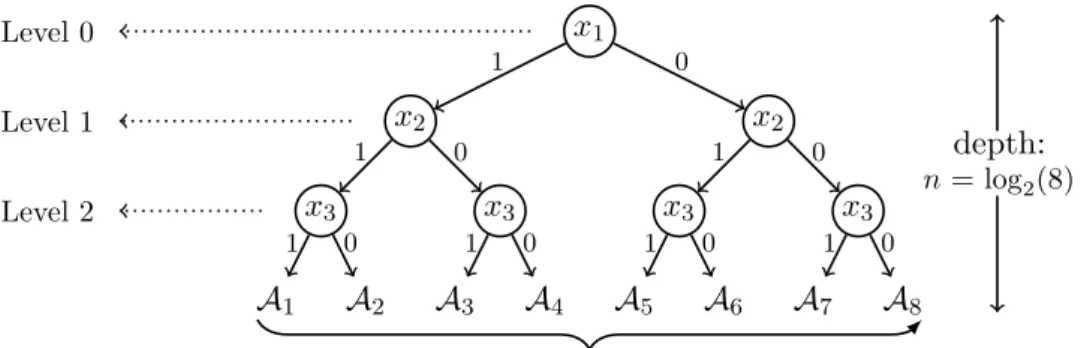
Figure 2.1. A search tree of enumerating all truth assignments over Boolean variablesx1, x2 andx3in decision variable order−−−−→x1x2x3 which corresponds the decision levels from top to bottom in the leftmost of figure.

Figure 2.1 depicts a search tree that enumerates the truth assignments over Boolean variablesX ={x₁, x₂, x₃}indecision variable order−−−−→x₁x₂x₃. Decision levels (starting from level 0) of each assignment reflects this order. The observation about this tree is that it essentially is ann-depthcomplete binary tree, wheren=|X|, i.e., the number of variables, and its leaves are in one-to-one correspondence with the truth assignments under consideration. Hence, testing satisfiability can be viewed as a process of searching for a leaf node that satisfies the given CNF. Obviously, a brute-force search for all possible assignments is in O(2ⁿ). The decision level associated with variables used for branching steps (i.e., decision assignments) is specified by the search process, and denotes the current depth of the decision stack.

A DPLL explores the tree using depth-first-search algorithm, which incorporates unit propagation (UP), also calledunit resolution. Given our notational conventions in Definition 1, a CNF F is satif F =∅. Moreover, F is unsatif ∈ F. These two properties correspond to common boundary conditions that arise in recursive algorithms on CNF. In general, a CNF F is said to imply another CNF Γ, denoted F |= Γ, iff every assignment that satisfies F also satisfies Γ. Note that if a clauseCi

is a subset of another clause Cj,Ci ⊆Cj, then Ci |=Cj. We say in this case that clause C_i subsumes clause C_j, as there is no need to have clause C_j in a CNF that also includes clause Ci. One important fact based on this discussion is that F is intrinsically unsatifF |=.

2.1 The DPLL Algorithm 17

2.1.1 Unit propagation

Example 6. Consider the following CNF:

F = (x₁∨x₂∨x₃)∧(¬x₁∨ ¬x₃)∧(¬x₂∨x₃)

Consider also the node at Level 1 on the left branch as shown in Figure2.1, which results from assignmentA(x₁) = 1, and we have:

A(F) = (¬x₃)∧(¬x₂∨x₃) (2.1) Currently, F is neither empty (∅), nor includes the empty clause (). Therefore, we cannot yet declare early success (sat) or early failure (unsat), which is why a brute-force algorithm continues searching below Level 1.

However, that by employing UP, we can indeed declare success and end the search at this node. Firstly, we close F under UP and collect all unit clauses² in F. Then we assume that literals are assigned to 1 to satisfy these unit clauses.

Lastly, we simplify F given these assignments and check for either that all clauses are subsumed or that the empty clause is derived.

To incorporate UP into DPLL algorithm, we introduce a function UnitPropa- gate, which applies to a CNFF and returns two results:

• L: a set of literals that were either present as unit clauses inF, or were derived fromF by UP.

• Γ: a new CNF which results from assignments forF on literals Lconditioning to assign all of them to 1. Notationally, Γ =A(F)| ∀l(l∈ L) (A(l) = 1).

Continuously consider Formula 2.1, we have L={¬x₃,¬x₂}and Γ =∅.

UP is a very important component of search-based SAT solving algorithms because of its efficiency that we can apply all possible UP steps in time linear in the size of given CNF. DPLL is a refinement on depth-first-search which incorporates UP as given in Algorithm1. Beyond applying UP on Line1, we have two additional changes to ordered brute-force search as shown in Figure 2.1. First of all, we no longer assume that variables are examined in the given decision variable order as we go down the search tree. Secondly, we no longer assume that a variable is assigned to 1 first, and then to 0; see Line5. The particular choice of a literal ls.t. l∈Γ can have a dramatic impact on the running time of DPLL. Many heuristics have been proposed for making this choice. Among them, a quite effective heuristic, well-known as variable state independent decaying sum (VSIDS) attempts to score each variable and select thevariable polarity (corresponding to literal and its negation) with the highest score to determine where to branch [55].

2.1.2 Chronological backtracking

DPLL (Algorithm1) is based on chronological backtracking. That is, if we try both values of a variable at Levelt, and each leads to a contradiction (conditional unsat),

2 If a clause only contains a single literal, then it is called a unit clause.