SAHDEV KUMAR

DEVELOPMENT OF A LONG-RANGE ULTRASONIC IMAGING SYSTEM IN AIR

USING AN ARRAY TRANSMITTER

SAHDEV KUMAR

A Thesis for the Degree of

‘Doctor of Engineering’

DEVELOPMENT OF A LONG-RANGE ULTRASONIC IMAGING SYSTEM IN AIR

USING AN ARRAY TRANSMITTER

Graduate School of Engineering

ELECTRICITY AND MATERIALS ENGINEERING COURSE AICHI INSTITUTE OF TECHNOLOGY

MARCH 2017

SAHDEV KUMAR

_____________________________________

Contents

______________________________________

Chapter 1: Introduction

1.1 What is ultrasonic sound? --- 1

1.2 Applications of ultrasonic sound --- 2

1.3 Techniques available for 3D measurement --- 4

1.3.1 Stereo camera --- 4

1.3.2 Laser scanner --- 5

1.3.3 Pattern projection --- 6

1.4 Overview of ultrasonic imaging sensor system --- 6

1.4.1 Phased array system --- 7

1.4.2 Principle of ultrasonic imaging sensor system --- 7

1.4.3 Types of imaging sensor system --- 8

1.4.4 Issues concern ultrasonic imaging sensor system --- 10

1.4.5 Signal processing for resolution --- 12

1.5 Sound field divergence of single transmitter --- 14

1.5.1 Concept of array transmitter --- 16

1.6 Purpose of this work --- 16

1.7 Composition of thesis --- 17

References --- 19

Chapter 2: High Power Ultrasonic Transmitter Array for 3-D Range Imaging.

2.2 Theory --- 23

2.2.1 Continuous wave --- 23

2.2.2 Pulse modulation --- 29

2.2.3 Measurable range --- 34

2.3 Transmitter array structure --- 35

2.4 Experimental set-up --- 37

2.5 Experimental method --- 38

2.6 Experimental results --- 39

2.6.1 Characteristics of array transmitter --- 39

2.6.2 Pulse modulation and sound pressure level --- 42

2.6.3 Pulse modulated directivities --- 43

2.7 Conclusion --- 45

References --- 45

Chapter 3: Long-Range Measurement System Using Ultrasonic Transmitter Array and Range Sensor in Air

3.2 Ultrasonic transmitter array --- 49

3.3 Ultrasonic receiver array --- 49

3.4 Principle of object detection --- 57

3.5 Experimental set-up --- 58

3.6 Experimental results --- 59

3.6.1 Measurable range --- 59

3.6.2 Image detection --- 61

3.7 Conclusion --- 65

Reference --- 66

Chapter 4: Isotropic Divergence Controllable Ultrasonic Transmitter Array for 3-D Range Imaging

4.2 Theory --- 69

4.3 Structure of divergence controllable transmitting system --- 76

4.4 Experimental results --- 78

4.4.1 SPL at different divergence --- 78

4.4.2 Directivities at different divergence --- 79

4.4.3 Measurable range --- 81

4.4.4 Image detection --- 82

4.4.5 Object detection view angle --- 87

4.5 Conclusion --- 88

References --- 89

Chapter 5: Anisotropic Divergence Controllable Ultrasonic Transmitter Array for 3-D Range Imaging

5.2 Theory --- 92

5.3 Structure of divergence controllable transmitting system --- 99

5.4 Experimental results --- 100

5.4.1 SPL of array transmitter with anisotropic divergence --- 100

5.4.2 Directivities with anisotropic divergence --- 101

5.4.3 Measurable range using anisotropic divergence --- 103

5.4.4 Detection of range image --- 104

5.5 Conclusion --- 107

References --- 108

Chapter 6: Summary

Scope of the future work

List of papers

Acknowledgement

1

Chapter 1

______________________________________

Introduction

______________________________________

1.1 What is ultrasonic sound?

Ultrasonic sound wave investigations involve the study of sound waves propagating at frequencies beyond the human audible range from 20 to 20,000 Hz. Very high frequency sound waves above the limit of human hearing were generated by English scientist Francis Galton in 1876, through his invention, the Galton whistle.

Even though piezoelectric and magnetostrictive effects were known but they were not utilized in any useful ultrasonic instruments due to lack of progress in electrical technology and hence Galton’s work showed negligible curiosity for over three decades on ultrasonic instrument application.

However, the experiences of world war during 1914-1918, attracted interest in the subject when French physicist Paul Langevin and Russian scientist Chilowsky, developed a powerful high frequency ultrasonic echo-sounding device, called ‘hydrophone’ in France. The hydrophone was further improved in classified research activities and deployed extensively in the surveillance to detect the submarines as well as under water communication in 1916.

It was felt that rapid growth in the field of electronics after world war-I was the need of time. In 1925, Pierce used quartz and nickel transducers for generating and detecting ultrasonic sound frequencies extending up to MHz range. By the time, Debye and Sears as well as Lucas and Biquard, independently discovered the ultrasonic diffraction grating to boost the steady progress in the use of ultrasonic sound to study the acoustical properties of liquids and gases. And by the 1930s, ultrasonic investigations

2

into the properties of solids were being done. A Soviet scientist Sokolov, is considered as the father of ultrasonic testing and published details of the experimental design of quartz generators, methods of coupling the generators to the test piece in order to achieve maximum energy transfer, and also various methods of detecting the ultrasonic energy after transmission through the test piece in 1935. Moreover, the scope of ultrasonic sound has been enhanced considerably by adopting pulse methods derived from Radio Detection and Ranging (RADAR) techniques, and, it has been widely applied in, e. g., the non-destructive testing of materials, medical diagnosis, and instrumentation and control applications. Other potential uses of high intensity ultrasound including cleaning, emulsification, drilling, sub-micro and micro material processing methods could also be realized.

New materials and techniques were discovered in 1960s and with the developments of microwave propagation, it could possible to generate ultrasonic waves at frequencies up to 100 GHz for its further applications in fundamental research in physics, electronic communications and computer technology.

The ultrasonic use is preferred to audible sound in various applications owing to the following reasons:

1. Ultrasonic sound has directional properties, with greater directivity at higher frequencies and is suitable for flaw detection and underwater signalling.

2. Higher frequencies means “shorter wavelengths”, i.e., less than or equal to the samples of the material for propagation, is important for small thickness measurement and high resolution flaw detection.

3. Ultrasonic sound is silence and hence makes it advantageous in high intensity applications. Such applications are possible with higher efficiency at audible frequencies, but resulting noise may be intolerable and possibly injurious.

Ultrasonic applications are classified based on either low or high intensity.

3

Low intensity ultrasonic waves are normally used either for investigating the properties of material samples which do not change its structural and chemical properties or control methods. Most low intensity ultrasonic wave applications involve very high frequencies, typically in MHz range, with the acoustic power involved might be from a few microwatts (W) to several tens of milliwatts (mW). On the other hand, high intensity ultrasound is used for changing the properties of material through which it is passed. Often high intensity ultrasonic wave frequencies are just above the audible limit, with the acoustic power involved from a few mW to kW. Ultrasound with its frequency range is used for various functions. A categorization of ultrasound with its functions is shown in Fig. 1.1.

Fig. 1.1: Ultrasound applications as per frequency range

1.2 Applications of ultrasonic sound

The most common use of ultrasound is in ultrasonic imaging and at present most widely used for bio-medical applications. Ultrasound also has a number of other industrial applications such as image processing, inspection modalities, three-dimensional (3D) imaging etc. Their use in creating images is based on the reflection and transmission of the ultrasonic pulsed wave at a boundary. When an ultrasound wave travels inside an object that is made up of different materials (such as the human body), each time it encounters a boundary (e.g., muscle and bone or muscle and fat); a part of the ultrasonic wave is reflected while as other part gets transmitted. The reflected ultrasonic pulsed waves are detected and used to construct an object image.

4

Ultrasound is also used in RADAR and Sound Navigation and Ranging (SONAR) technologies; both of which work on the same principle in which the ultrasound pulses is transmitted in the form of short burst with the fixed interval, which gets partially reflected back from the target and received back by the receiver. Some creatures such as Bats and Dolphins also use ultrasound to find out their prey based on the principle of finding an object distance using an ultrasonic sound wave reflection, called “echo”. If the speed of sound in the medium is known, then object distance can be obtained.

The time required for an echo to return, is calculated and converted into distance for the known speed of sound in that medium.

1.3 Techniques available for 3D measurement

There are some other techniques also used for 3D measurements of any object, namely

1. Stereo Camera 2. Laser Scanner 3. Pattern Projections 1.3.1 Stereo camera

Some latest models of Stereo Camera are available in the market and their working principle is shown in Fig. 1.2, in which two cameras with parallel optical axes placed at the distance d between them and line connecting the camera lens centres is considered as baseline. This baseline is perpendicular to the line of sight of both the cameras. X axis of the 3D coordinate system is parallel to the baseline. The origin O lies in mid-way between the lens centre and with the coordinate geometry, image of point P is obtained.

Limitations of the stereo camera

Stereo camera can measure accurately for short range only. The disparity and corresponding point’s image matching are the main drawback of this system.

5

Fig. 1.2: Working principle of stereo cameras.

1.3.2 Laser scanner

Another technique used for 3D measurement is light amplification by stimulated emission of radiation (LASER) scanner. There are many devices that can be called 3D scanners. Any device that measures the physical world using lasers, lights or x-rays and generate dense point clouds or polygon meshes can be considered as a 3D scanner. They are also known as 3D digitizers, laser scanners, white light scanners, industrial computed tomography (CT), light detection and ranging or laser imaging detection and ranging (LIDAR) etc. The common uniting factor of all these devices is that they capture the geometry of physical objects with hundreds of thousands or millions of measurements. Fig 1.3 shows the measurement method of scanner.

Limitations of scanner

Scanners are suitable for medium range only and long range measurement is not possible. The experimental results of this technique are not reliable due

Object Surface P(x,y,z)

Base

o

d ^{(x’r, y’r)}

(x’l, y’l⁾

Right Camera Left Camera

6

to higher noise and slow data acquisition.

Fig. 1.3: Measurement method of scanner.

1.3.3 Pattern projection

Pattern projection is also used for 3D measurement of an object in air. In this technique structured light generates a full pattern to cover the object so that the surface can be captured as whole field recording. The encoding of structured pattern becomes important because it determines the local feature of the recorded images that to be identified in spatial recognition and height evaluation.

Limitations of pattern projection

Pattern projections are fast and long range measurement is possible if both resolution and robustness are high.

1.4 Overview of ultrasonic imaging sensor system

An ultrasonic imaging sensor system has the following merits over other conventional techniques. First of all its constructions is simple, second it is one of the fastest measurement technique, third it maintains the privacy while

7

monitoring human daily activities and last this technique is useful in adverse atmospheric conditions such as rain, fog, smoke, darkness etc.

1.4.1 Phased array system

Conventional ultrasonic transducers for Non-Destructive Testing (NDT) commonly consisting of either a single active element that both generates and receives high frequency sound waves, or two paired elements, one for transmitting and one for receiving. Phased array probes, on the other hand, typically consists a number of transducer and each one of them can generate pulses separately. The elements may be arranged in a strip (linear array), a ring (annular array), a circular matrix (circular array), or any other more complex patterns. In range sensing system low frequencies is used. A phased array system will also include a sophisticated computer-based instrument that is capable of driving the multi-element probe, receiving and digitizing the returning echoes, and plotting that echo information in various standard formats. Unlike conventional flaw detectors, phased array systems can sweep a sound beam through a range of refracted angles or along a linear path, or dynamically focus at a number of different depths, thus increasing both flexibility and capability in inspection setups.

1.4.2 Principle of ultrasonic imaging sensor system

In ultrasonic range imaging sensor system an electric signal of known frequency above the human audible limit > 20 kHz is generated in the form of modulated pulse and received back by an ultrasonic receiver after reflection from an object. The electrically generated ultrasonic signal is converted to analogue signal from its digital form through digital to analogue converter (DAC) before its transmission in air. The ultrasonic analogue signal is again converted into the digital form by an Analogue to Digital Converter (ADC) after its detection by the receiver for signal processing such as the auto correlation function.

8

Fig. 1.4: Linear array receiver for measuring the angle  of the target based on the difference in arrival time ∆T = ^∆𝑅

𝑐 between adjacent elements.

In order to find the direction of the target object from the transceiver, an angle measurement system is needed. A linear array of receivers is used to receive a plane wave reflected from the object as depicts in Fig. 1.4. An incident angle  creates a difference in the Time-of-flight between neighbouring elements with the following relationship as given by Eq. (1.1) [6-7]

∆𝑇 =

𝑐

sin⁡(𝜃)

Here, d and c denote the inter element space and sound wave velocity respectively. That corresponds to a phase shift ∅ =^2𝜋𝑑_ sin (),  is the wavelength. In the same way, to transmit a pulse with the angle  from normal, the phase of the transmit signal should be shifted by  between each element.

1.4.3 Types of imaging sensor system

9

Generally, imaging sensor system can be classified in two types (i) Scanning method

Scanning method is widely used in medical and underwater imaging and not good for long range measurement. Therefore, for long range measurement non-scanning method is useful. They have the merit of fast measurement but low resolution and measurable range. Scanning method has the opposite characteristics being slower but having high resolution and long measurable range [1-3].

(ii) Non-scanning method

This non-scanning method can be further divided in two types (a) Holographic

Holography is a branch of optics used for recording and displaying an image.

The two concepts, interference and diffraction are commonly used in optics and their combined form make a single branch called holography and optical data processing. Interference and diffraction in communication terminology are known as modulation and demodulation. It became possible that information stored in an interference pattern (modulation) can be recorded as a result of diffraction of light by the recorded interference pattern (de- modulation) [4, 5].

(b) Beam forming of receiver

(i) Delay-and-sum Beamforming

The delay-and-sum beamforming is the simplest techniques for realizing directional array systems and also knows as classical beamforming. Initially delay-and-sum arrays were used in narrowband operation to focus arrays in a particular direction. Narrowband beamforming is generally implemented with the phase shifts and is referred as phased-array beamforming. The

10

delay-and-sum beamforming uses delays between each array element that compensate for differences in the propagation delay of the desired signal direction across the array. The signals generating from a desired direction are summed in phase and others becomes null due to destructive interference.

The shape of the beam and side lobes along with the position of the nulls of the array can be controlled by adjusting the weights of the delay-sum beam former.

(ii)Delay-and-multiplication Beamforming

Delay-and-multiplication operations are used to increase the sharpness of main lobe.

1.4.4 Issues concern ultrasonic imaging sensor system

Although, ultrasonic range imaging system has several advantages over other conventional methods but it has some drawbacks also such as bigger size, ghost image, low resolution and low measurement range etc. These drawbacks are being eliminated as discussed below

(a) Size

The one of the major drawback of imaging sensor system is the bigger size of the array receiver. This drawback has been resolved with the recent development of Micro Electro Mechanical System (MEMS) through which it became possible several tens and/or several thousand receivers can be adjusted in a very small area. The real through of imaging sensor system is the development of MEMS technology that significantly reduces the size. An integrated circuit has been developed that consist of single transmitter and array receiver in a single chip [6, 7]. Further, an array receiver has been constructed using PZT thin film [8, 9].

(b) Ghost image

Another drawback of the imaging sensor system is obtaining ghost images.

It is due to the large inter-element space of the array receiver than that of the

11

wave length of the ultrasonic sound. The ghost images appear due to the strong reflected signal from other objects located in different direction. The grating lobes and side lobes cause ghost image. This drawback is resolved reducing the inter-element space of microphones using the MEMS technology. An array receiver that composed of total eight small area and each small area consists of four receivers. After delay-and-sum operations, delay-and-multiply operations are applied on the received signal. Such receiver decreases the grating lobes and side lobes thus eliminating the ghost image. [10-11]. Further attempt has been made by increasing the number of element in the receiver array and arranging them in different patterns [12].

The pitch of the side lobe is calculated by Eq. (1.2) as follows [4]

sin𝜃

=

(𝑛−1)𝑑 (1.2)

Where, d is the pitch of the elements, n is the number of elements, and m is the order of the side lobes. Since elements are placed at 10 mm intervals, the number of elements is 12, and the wavelength of the ultrasonic wave is 8.6 mm, side lobes with a pitch of 4.5, or 0.078 radians [= 8.6 mm/10 mm × (12-1)], appear at lower angles. Grating lobes appear at an angle using Eq.

(1.3) as follows

sin𝜃

=

𝑑 (1.3)

Where, m’ is the order of the grating lobes. The pitch becomes sin⁻¹(^{8.6⁡ mm}

10⁡ mm) = 1.0⁡ rad. = 60⁡ deg.

(c) Resolution

Resolution is another drawback of the imaging sensor system due to the large number of array receivers used in the system. This drawback has been resolved using the dispersed ultrasonic array receiver and applying the delay- and-multiply operations (H. Furuhashi et al.) [13]. The camera image has been taken into consideration to improve the resolution along with the array receiver. [14, 15].

12

(d) Measurable range

Ultrasonic sound is absorbed by the air, therefore measurable range is limited to a few meters only. Some efforts have been made to improve the measurable range such as

(i) Increasing the number of transmitting elements

Measurable have been improved up to 15 m by increasing the number of transmitting element and developing the high power transmitter array. With this system measurable range improved significantly and the directivity of transmitter array becomes very narrow [16-18].

(ii) Using electric spark discharge

Another attempt to increase the measurable range is development of electrical spark discharge. Measurable has been improved over 5 m with this method and object detection view angle also present up to a few degrees. With this system high power sound is generated by short circuit. This method is dangerous and someone may get injured.

Further, one can loss his eyesight due to sparking [19, 20].

(iii) Spread spectrum pulse compression technique

Using the spread spectrum pulse compression technique, we have successfully increased the S/N ratio, therefore, measurable range improved up to 8 m. Object detection view angle up to a few degree is also obtained [21-23].

(iv) Acoustic lens

Using acoustic lens, measurable range up to 6 m has been reported and object detection view angle is present to a few degrees [24].

1.4.5 Signal processing for resolution

Before the discussion of aperture synthesis or super resolution, it is equally important to address the need to make proper use of acoustic aperture for high resolution. Let us consider a one-dimensional aperture containing ‘n’

13

equally spaced liner detectors or ‘n’ equally spaced sampling points, then there are ‘2n’ of input information, phase and amplitude for each frequency band. If this is processed to form an image using, i.e. Fast Fourier Transform (FFT), it ends up with ‘2n’ output words of information including phase and amplitude and no loss of information is expected. Although, most imaging systems only display intensity and thus ‘n’ of information is the final output and half of the information get lost. By Rayleigh criteria, it may be readily seen that there should be twice as many points in the intensity display, spaced half as far as in a phase display. It ends up with the required ‘2n’ output and the full resolution capability of the acoustic aperture which is being used.

It is observed that the two sources cannot be resolved in the 20 x 20 pixel intensity display, even they are in out of phase and their separation is also greater than Rayleigh distance. After interpolation to obtain the display in 40 x 40 pixels, the two sources are clearly resolved. There are two methods for processing the interpolation (a) Synthetic-aperture processing (b) Super resolution processing [30-34].

(a) Synthetic-aperture processing: This processing is possible by two ways (i) The receiver aperture is synthesized by motion of either the object, or

the receiver, or the transmitter, or any two of these.

(ii) The receiver aperture is synthesized by multiplexing transmitters, so that no motion is involved.

(b) Super resolution processing

A method has been proposed by Gerchberg [29] is designed to be more robust against noisy environments. This approach, is called the error-energy reduction method, is an extension of Harris method [27, 28]. In this method, the input (far-field holographic) data are first Fourier transformed to yield the conventional image. The image is then modified by setting all of the image points outside the known extent of the true object to zero. The image thus modified is Fourier transformed to form a far-field hologram over a larger aperture than originally available, with the original hologram data being substituted only where it was available (i.e., over the original aperture)

14

and the new data being used outside this region.

These steps are repeated until a criterion based on the estimated object energy outside the known extent of the true object is satisfied and known as converge. The range image resolution depends on the signal bandwidth. The shorter pulse width modulation has larger bandwidth and gives better range image resolution. The bandwidth limitations are imposed by the bandwidth of the transmitters or receivers as they are resonant devices. The range image resolution could be improved using pulse compression technique [35-37].

When a short modulated pulse incidents on the receiver array at an angle, it does not reach all the elements of the array receiver at the same time.

Therefore, time-delay beam-forming is used, as a result some of the outer elements are completely missing the pulse, reducing the resolution for off- axis objects. This effect has been analysed and does not have serious effect [38-41].

1.5 Sound field divergence of single transmitter

It is necessary to understand the sound field radiation by a single element transmitter before designing a phased array transmitter. Single element transmitter`s sound field characteristics are calculated with the following considerations; (i) The size and shape of the transmitting element (ii) The transmitted pulse properties and (iii) The characteristics of the medium of propagation.

The rate at which the energy in this region diverges is a function of the source diameter (D), the radiated wavelength () and () is the absorption coefficient.

The highest amplitude signal occurs on the axis of the transducer and amplitude decreases on the angular displacement from the axis as shown in Fig. 1.6. Although the signal is radiated into the entire half space, most of the energy is included in this conical far field region. The lateral limits of this cone is defined as the angle at which the signal amplitude is reduced by 6 dB relative to the axial amplitude and angle at which the signal amplitude is reduced by 6 dB and calculated by the Eq. (1.4)

15

) 7 . 0 1 (

sin D

    

(1.4)

It can be observed that when  (wavelength) is large in comparison to D (diameter), the divergence is large. It makes the object positioning of the reflector more difficult due to the larger sound field. Therefore, during inspection of the quality of the material, ultrasound transmitters having small divergence angle are preferred, so that the reflector can be located more precisely. This divergence angle can be reduced by reducing the ratio of /D in the Eq. (1.3). There are two methods to reduce the divergence angle; (i) producing the higher frequency or increasing the diameter of the transmitter and (ii) Focusing the ultrasound source itself but it is not possible using single transmitter.

In some of the applications we required small divergence angle such as inspection of quality of material and detection of fault in a product. On the other hand in some applications wide divergence angle is required such as 3D range imaging. Ultrasound source cannot be focused using single transmitter, therefore concept of array transmitter has been proposed [25, 26].

Fig. 1.6: Directivity pattern of single transmitter.

0°

15°

30°

15°

30°

0°

15°

30°

15°

Small /D 30°

Large /D

16

1.5.1 Concept of array transmitter

The measurable range using conventional ultrasonic method is limited due to the fundamental characteristics of ultrasonic waves. Thus high power array transmitters could be used in non-destructive evaluations and inspection modalities. Also, measurable range of the 3D image sensor may be improved using such type of array transmitter owing to their high sound pressure level. With this consideration, a high power ultrasonic transmitter array (UTA) has been developed.

With increased use of ultrasonic testing and measurements in past several years, such as scanning techniques for both contact and immersion method during production and in-service inspection programs to determine the quality of the product. Due to a variety of component configurations and potential flaw geometries it is often necessary to perform several inspections each with a different probe configuration to assure the defect findings, if any.

A purposely designed phased array probe can perform various inspections without changing hardware to sufficiently reduce the inspection time.

Using array structure following functions can be performed

 Ultrasonic sound source can be focused

 Isotropic divergence control is possible on ultrasonic sound source

 Anisotropic divergence control is possible on ultrasonic sound source 1.6 Purpose of this work

Due to the fundamental properties of ultrasonic sound, the conventional ultrasonic range imaging system is restricted to measure 3D position of an object only up to a few meters. Therefore, main focus remained to improve the measurable range. The measurable range could be improved up to 8 m by spread spectrum pulse compression method when a steel plate (10 cm width x 12 cm length) has been used as an object and detected accurately [22].

A high power sound source also has been developed by spark discharge [20]

and measurement range has been improved over 5 m. This method is dangerous for the safety point of view and one can suffer for permanent

17

hearing loss or visibility.

Keeping in mind the above factor, a safe and convenient method was the primary requirement for the development of high power sound source.

Therefore, a high power ultrasonic transmitter array has been constructed.

With the development of high power sound source, measurable range is expected to be improved. With this idea, that high ultrasonic power can be maintained for long distance, an ultrasonic transmitter array has been developed.

This work has undertaken owing to the fact that in last few decades the applications of ultrasound has been increased to a great extent. A high power UTA for 3D range imaging system would improve the scope of ultrasonic sound applications not only in the advanced fields of control engineering, security, alignment, flaw detection, robotics, amusement, sub-micro and micro material processing industrial utilities etc. but also in bio-medical science and engineering.

The ultrasonic imaging sensor system is a simple and cost effective technique for 3D position and shape recognition of an object. Additional advantage of this system is that it is useful in adverse atmospheric conditions. Before developing such system, minutely all the point must be borne in mind to optimise the performance of the system. With the concept of transmitter array, it could be possible to focus the sound source. The main focus of this work are as follows

 Improvement in measurable range over 15 m.

 Improvement in the object detection view angle over 15^o. 1.7 Composition of thesis

In order to improve the measurable range, a 2D transmitter array has been proposed that can generate high power. Therefore, a high power ultrasonic transmitter array has been constructed. In this dissertation, a long range imaging sensor system using high power array transmitter is being reported and explained in chapter wise. This thesis composed of 6 chapters as follows.

18

In Chapter-1, background of the field of range imaging sensor is described and make comparisons with other conventional techniques for 3D measurement of an object with the range imaging sensor system using ultrasonic sound. The motivation and purpose of this study is also described.

Chapter-2 describes about the principles and configurations of the array transmitter. The characteristics of the transmitter on the number of elements, modulated pulse width etc. is investigated theoretically. Experimental investigation is also performed and compared with the theoretical results.

The performance of the transmitter on range imaging system is also discussed theoretically.

Chapter-3 presents principle and configuration of the long-range measurement system using UTA and URA. The experimental studies were conducted on the measurable range using (i) single ultrasonic transmitter (SUT) with single ultrasonic receiver (SUR) (ii) SUT with ultrasonic receiver array (URA) (iii) UTA with SUR (iv) UTA with URA and compared their performances.

Chapter-4 describes the improved 3D measurement field of an object by controlling the sound divergence of the UTA to improve the object detection view angle of the system. The coordinate system of the divergence control of UTA and the configuration of the system have been explained. The characteristics of the transmitter is investigated theoretically and compared with experimental results. A range imaging system using this transmitter and ultrasonic receiver array is constructed. The performance of the system is investigated and compared with the system using the ultrasonic array transmitter without the sound divergence control.

Chapter-5 discussed the range imaging system using UTA with anisotropic divergence control. In some particular cases a wide horizontal field and narrow vertical field is required for measurement. With anisotropic divergence control system, independent control on horizontal and vertical divergence is possible. The principle and the configuration both are described in detail. The characteristics are investigated theoretically and

19

compared with the experimental results. The performance of the range image sensor system using UTA, has been discussed and compared with the system using UTA without sound divergence control and that with the isotropic divergence control.

Chapter-6 summarizes this dissertation. Further, scope for the future research work is also given.

References

[1] L. Azar, Y. Shi and S.C. Wooh, Beam focusing behavior of linear phased arrays, NDT & E International, 33, (2000), pp. 189-198

[2] Y. Lu, H.Y. Tang, S.Fung, B.E. Boser and D.A. Horsley, Pulse-echo ultrasound imaging using an A1N piezoelectric micromachined ultrasonic transducer array with transmit beam-forming, J.

Microelectromechanical systems, 25 (1) (2016), pp.179-187.

[3] E. Konetzke, M. Rutsch, M. Hoffmann, A. Unger, R. Golinske, D. Killat, S.N. Ramadas, S. Dixon and M. Kupnik, Phased array transducer for emitting 40-kHz air-coupled ultrasound without grating lobes, Proc.

IEEE Ultrasonics Symposium, 2015, IEEE Xplore, DOI:

10.1109/ULTSYM.2015.0019 (2015).

[4] A. Korpel, Acoustic imaging and holography, IEEE Spectrum, 52 (1968), pp.45-52.

[5] Dunn F. et al., Springer handbook of acoustics, Ed. Thomas Rossing.

Springer (2015).

[6] R. J. Przybyla, H. Y. Tang, A. Guedes, S. E. Shelton, D. A. Horsley and B. E. Boser, Digital ultrasonic rangefinder on a chip, IEEE Journal of Solid-State Circuits, 50 (1) (2015), pp.320-334.

[7] R. J. Przybyla, S. E. Shelton, A. Guedes, R. Krigel, D. A. Horsley and B.

E. Boser, In-air ultrasonic range finding and angle estimation using an array of ALN Micromachined transducers, IEEE Sensors, J. 11 (11) (2011), pp.2690-2697.

[8] K. Yamashita, L. Chansomphou, H. Murakami and M. Okuyama, Ultrasonic micro-array sensors using piezoelectric thin films and resonant frequency tuning, Sensors and Actuators A 114 (2004), pp. 147- 153.

20

[9] K. Yamashita, H. Katata, M. Okuyama, H. Miyoshi, G. Kato, S. Aoyagi and Y. Suzuki, Arrayed ultrasonic microsensors with high directivity for in-air use using PZT thin film on silicon diagrams, Sensors and Actuators Acous. Physical 97-98 (2002), pp. 302-307.

[10] H. Furuhashi, Y. Uchida and M. Shimizu, Imaging sensor system using rectified delay-and-multiply operations with an ultrasonic array, Industrial Electronics 2008, IECON 2008 (2008), pp. 1891-1895.

[11] H. Furuhashi, Y. Uchida and M. Shimizu, Imaging sensor system using a composite ultrasonic array, IEEE Sensors 2009, IEEE Xplore (2009), pp.1467-1472.

[12] S. Harput and A. Bozkurt, Ultrasonic phased array device for acoustic imaging in air, IEEE Sensors Journal 8 (11) (2008), pp.1755-1762.

[13] H. Furuhashi, J.Valle, Y.Uchida and M. Shimizu, Imaging sensor system using dispersed ultrasonic array, Proc. of ICCAS 2007 (2007), FEP-35, pp. 2385-2388.

[14] H. Furuhashi, Y. Kuzuya, Y. Uchida and M. Shimizu, Three-dimensional imaging sensor system using an ultrasonic array sensor and a camera.

IEEE Sensors 2010, IEEE Xplore A2P-P4 (2010), pp.713-718.

[15] H. Furuhashi, Y. Kuzuya, Chen Gal, and M. Shimizu, Three- dimensional imaging of a human body using an array of ultrasonic sensors and a camera, 2^nd International conf. on Advances in intelligent and soft computing camera. 145 (2012), pp. 325-330.

[16] J. Majchrzak, K. Michalski and G. Wiczynski, Distance estimation with a long range ultrasonic sensor system, IEEE Sensors Journal, 9 (7) (2009), pp.767-773.

[17] Datashseet, 6500 series sensor ranging module, sens Corp, Inc. 2004, Dec.18 2007. [Online]. Available:www.senscomp.com /6500smtmod.htm.

[18] Datasheet, Technical specification for 600 series instrument grade electrostatic transducer, Polaroid 6/95, Sep. 8 2008. [Online]. Available:

www.engr.udayton.edu/faculty/jloomis/ece445/topics/sonar/6500.pdf.

[19] J. M. M Aberu, R. Ceres, C. Leopoldo, M.A. Jime’nez and P. Gonza’lez- de-Santos, Measuring the 3D-position of a walking vehicle using ultrasonic and electromagnetic waves, Elsevier Science S.A. Sensors and Actuators, 178 (1999), pp.131-138.

21

[20] T. Tanaka, S. Lee, M. Uno, K. Inoue, S. Aoyagi, K. Yamashita and M.

Okuyama, Improvement of ultrasonic micro array sensor using the amorphous fluorocarbon polymer film, the transactions of the institute of electrical engineers of Japan. A publication of sensors and micromachines society 127 (1) (2007), pp.7-13.

[21] Y. Zhenjing, H. Li, C. Lina, Improvement of measurement distance in multi-channel ultrasonic ranging systems thorough adaptive chaotic pulse position width modulation excitation sequences, Insight-Non- Destructive testing and condition monitoring 58 (7) (2016), pp. 324-330.

[22] H. Furuhashi, S. Kumar and M. Shimizu, Signal processing of a 3D ultrasonic imaging sensor that uses the spread spectrum pulse compression technique, Lecture notes in information technology, Proc.

2012 Int. Conf. on Future Information Technology and Management Science & Engineering FITMSE 2012, 14 (2012), pp.145-150.

[23] H. Inubushi, N. Takahashi, H. Zhu and K. Taniguchi, Ultrasonic 3D image sensor employing PN Code and Beam-forming Technologies, IEICE Trans. Acous. J90-A (6) (2007), pp.517-523.

[24] Sai Hou, Buren Mandula, Wei Quan, Sahdev Kumar and Hideo Furuhashi, Imaging of a wave reflected by an object using an acoustic lens in air, IMEKO XXI World Congress, in USB 5 pages. (2015).

[25] B.W. Drinkwater and P.D. Wilcox, Ultrasonic arrays for non-destructive evaluation: A review, NDT and E International, 39 (7) (2006), pp.525- 541, DOI: 10.1016/J. ndteint. 2006.03.006.

[26] A.J. Fenn, D.H. Temme, W.P. Delaney and W.E. Courtney, The development of phased-array radar technology, Lincoln Lab. Journal, Vol.

12, No. 2, (2000), pp. 321-340.

[27] F.J. Harris, Diffraction and resolving power, JOSA, Vol. 54, No.7 (1964), pp. 931-933.

[28] F.J. Harris, On the use of windows for harmonic analysis with the discrete Fourier-transform, Proc. IEEE, Vol. 66 (1978), pp. 51-83.

[29] R.W. Gerchberg, Super-resolution through error energy reduction.

Journal of Modern Optics, Vo. 21 No. 9 (1974), pp. 709-720.

[30] R.W. Schafer and L.R. Rabiner, A digital signal processing approach to interpolation, Proc. IEEE, Vol. 61, (1973), pp.692-702.

[31] G.J. Grevera and J.K. Udapa, An objective comparison of 3-D image interpolation method, IEEE Trans. Med. Imag., Vol. 17 No.4 (1998), pp.

22

642-652.

[32] R.K. Mueller, Advances in holography, vol.1, N. H. Farhat, Ed. New York; Marcel Dekker, (1975), p.45.

[33] R.F. Koppelmann and P.N. Keating, Three dimensional acoustic imaging, presented at the Eighth Int. Symp. On Acoustical Imaging, May30-Jun, Key Biscayne, Florida, (1978).

[34] H.P. Brucker, Cross-sensor beamforming with a sparse line array, J.

Acoust. Soc. Amer., vol.61, (1977), pp.494-498.

[35] H. Kolsky, stress waves in solids, Dover Publications, New York, (1963).

[36] W.C. Elmore and M.A. Heald, Physics of waves, Dover publications, New York, (1985).

[37] D. Royer and E. Dieulesaint, Elastic waves in solids I and II Springer Verlag, Berlin, (2000).

[38] L.M. Brekhovskikh, Waves in layered media 2^nd Edition, Academic press, New York, (1980).

[39] J.D. Achenbach, Wave propagation in elastic solids, Elsevier science publisher, Amsterdam, (1990).

[40] B.A. Auld, Acoustic fields and waves in solids 2^nd Edition Vol.1&2, Krieger publishing, Florida, (1990).

[41] K. Preston, Use of pattern recognition for signal processing in ultrasonic histopathology, NBS Special publication 453, Proc. Seminar on Ultrason.

Tissue Characterization, May (1975).

23

Chapter 2

______________________________________

High Power Ultrasonic Transmitter Array for 3-D Range Imaging

______________________________________

2.1 Introduction

Recently, 3D shape and size measurement of an object is one of the thrust areas and efforts are being made to improve the measurement range and resolution [7, 11]. There are several techniques available for 3D position and shape recognition such as stereo camera, laser scanners, pattern projections etc. have been discussed in the previous chapter with their merits and limitations. Ultrasonic imaging sensor system is also one such technique and works on pulse echo method. In spite of low resolution, this technique has several advantages over them. This technique can be used in adverse atmospheric conditions [3-10].

In this chapter, configuration of the ultrasonic transmitter array (UTA), its coordinate system and simulation directivity with different pattern of transmitter array and pulse modulation have been discussed. Experimental study has been conducted at room temperature considering the ultrasonic wave speed 345 m/s and compared with the theoretical calculations.

2.2 Theory

2.2.1 Continuous wave

First of all, ultrasonic sound from the array transmitter for continuous-wave transmission is discussed. The directivity of a circular ultrasonic transmitter is described by Eq. (2.1) [1, 2]

24

𝐷(𝜃) =

𝑘𝑎 sin 𝜃 (2.1)

Here, 𝜃 is the direction of the sound wave, 𝑘 is the wave number, 𝑎 is the radius of an element, and 𝐽₁ is the Bessel function of the first kind. The radius of an element is 4.3 mm, an ultrasonic frequency of 40 kHz, and the wave velocity is 345 m/s. If there are many transmitting elements at position Pi (xi, yi, 0) in the plane z = 0 directed toward the z axis as shown in Fig. 2.1, the total sound pressure from all the elements will be given by Eq. (2.2)

𝑝(𝑥, 𝑦, 𝑧) = ∑ 𝐷(𝜃

)𝐴

−2πi𝑟𝑖 𝜆

𝑟_𝑖

𝑖 (2.2)

Here, 𝑟_𝑖 is the distance between position Pi of the element and the observation point P(x, y, z), 𝜃_𝑖 is the angle between the z axis and the vector P_iP

⃗⃗⃗⃗⃗⃗ , and 𝐴_𝑖 is the amplitude. If point P is sufficiently far from the origin compared with the size of the array, Eq. (2.2) can be approximated as Eq.

(2.3)

𝑃(𝑥, 𝑦, 𝑧) = ∑ 𝐷(𝜃

)𝐴

𝑒

√(𝑥−𝑥_𝑖)²+(𝑦−𝑦_𝑖)²+𝑧²



√(𝑥 − 𝑥

)

+ (𝑦 − 𝑦

)

+ 𝑧

𝑛

𝑖=1

≈ 𝐷(𝜃)𝐴 1

𝑟 ∑ exp⁡(−2𝜋𝑖 𝑟 − 𝑥

𝑥

𝑟 − 𝑦

𝑥

 𝑟 ⁾

𝑛

𝑖=1

= 𝐷(𝜃)𝐴 1

𝑟 𝑒

∑ exp⁡(2𝜋𝑖 𝑥

𝑠𝑖𝑛𝜃

+ 𝑦

𝑠𝑖𝑛𝜃

 ⁾

𝑛

𝑖=1

25

|𝑃(𝑥, 𝑦, 𝑧)| = 𝐴

𝑟

𝐷(𝜃)| ∑

exp (2𝜋𝑖

) | ⁡ ⁡ ⁡ ⁡

Here, 𝑟 is the distance between the origin (i.e., the center of the array) and the observation point P(x, y, z), ⁡ 𝜃 is the angle between z axis and OP⃗⃗⃗⃗⃗ . The 𝜃_𝑥 and 𝜃_𝑦 are the angles between the OP⃗⃗⃗⃗⃗ and the yz & xz planes respectively. It is assumed that all the elements have the same sound pressure amplitude.

Fig. 2.1: The coordinate geometry for sound pressure calculations.

Fig. 2.2 shows the directivity of single element having a radius of 4.3 mm according to Eq. (2.1).

Transmitter Array

 Y

P(x, y, z)

Z X

O(0,0,0)

r



r



26

Fig. 2.2: Directivity of single transmitter.

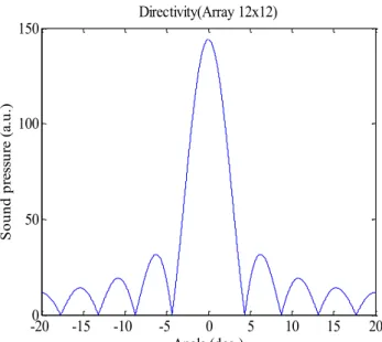
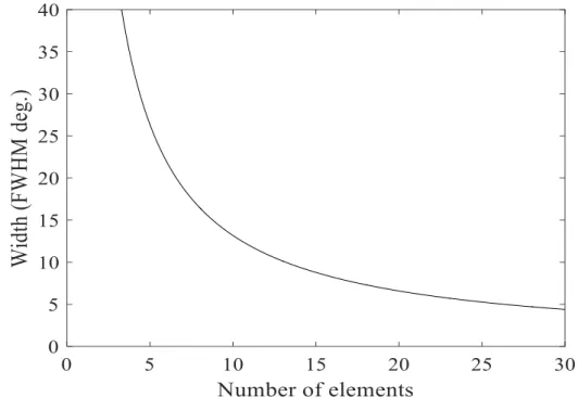
Fig. 2.3 shows the directivities calculated using Eq. (2.3). The elements having radius of 4.3 mm and 𝑛 × 𝑛 transmitting elements are located in square matrix with inter element space of 10 mm in the x and y directions.

Here, we assume⁡ ⁡ 𝜃_𝑥 = 𝜃; ⁡ 𝜃_𝑦 = 0, then. The sound pressure is normalized by 𝐴 𝑟⁄ , here A is the signal amplitude and r is the distance between center of array to the observation point . The sound pressure at the center (𝜃 = 0^𝑜) is directly proportional to the number of elements. The directivity increases with an increase in number of elements. Grating lobes appear at 𝜃 = 50 − 70° because the distance between each element (10 mm) is greater than the wavelength of the ultrasonic wave (8.6 mm). The simulation directivities with different pattern of transmitter array such as (2×2), (5×5), (10×10), (12×12) and (20×20) are shown in Figs. 2.3 (a)-(e). The directivity is about 5° (half width) for an array of (12×12) elements as shown in Fig. 2.4. The sound pressure 144 times higher than the single transmitter is obtained by this array transmitter.

-80 -60 -40 -20 0 20 40 60 80

0 0.2 0.4 0.6 0.8 1

Directivity

Angle (deg.)

Sound pressure (a.u.)

27

(a) (2×2) (b) (5× 5)

(c) (10× 10) (d) (12× 12)

(e) (20 ×20)

Fig. 2.3: Directivities with different pattern of Transmitter arrays.

-80 -60 -40 -20 0 20 40 60 80

0 1 2 3 4

5 Directivity(Array 2x2)

Angle (deg.)

Sound pressure (a.u.)

-80 -60 -40 -20 0 20 40 60 80

0 5 10 15 20 25

30 Directivity(Array 5x5)

Angle (deg.)

Sound pressure (a.u.)

-80 -60 -40 -20 0 20 40 60 80

0 20 40 60 80 100

Directivity(Array 10x10)

Angle (deg.)

Sound pressure (a.u.)

-80 -60 -40 -20 0 20 40 60 80

0 50 100 150 200 250 300 350 400

450 Directivity(Array 20x20)

Angle (deg.)

Sound pressure (a.u.)

28

Fig. 2.4: Directivity of ultrasonic array transmitter with (12×12) elements. The sound pressure is normalized by 𝐴 𝑟⁄ .

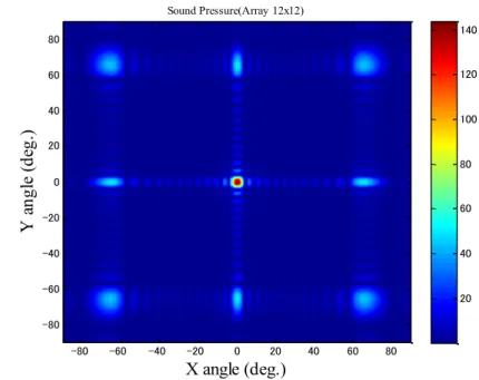
Fig. 2.5 shows a two-dimensional color map of the sound pressure for the directions 𝜃_𝑥 and 𝜃_𝑦. There are many side lobes along the 𝜃_𝑥 and 𝜃_𝑦 directions. The side lobes are small in other areas. Fig. 2.6 shows the directivity of (12× 12) array transmitter in the direction 𝜃_𝑥 = 𝜃_𝑦 . In this case

tanθ = √(tan 𝜃

)

+ (tan 𝜃

)

⁡ ⁡ = √2 tan 𝜃

The side lobes become small and the directivity becomes slightly large due to the short average distance of the elements in this direction.

-200 -15 -10 -5 0 5 10 15 20

50 100

150 Directivity(Array 12x12)

Angle (deg.)

Sound pressure (a.u.)

29

Fig. 2.5: Two-dimensional image of sound pressure. Ultrasonic array transmitter has (12×12)elements. The sound pressure is normalized by 𝐴 𝑟⁄ .

(a) -90^o to 90^o (b) -20^o to 20^o

Fig. 2.6: Directivity of ultrasonic array transmitter with (12×12) elements. The sound pressure is normalized by 𝐴 𝑟⁄ .

2.2.2 Pulse modulation

The range sensors, employ pulse-modulated wave and detect the distance of the object by the pulse echo method using time-of-flight (ToF). This section

X angle (deg.)

Y angle (deg.)

Sound Pressure(Array 12x12)

-80 -60 -40 -20 0 20 40 60 80

-80 -60 -40 -20 0 20 40 60 80

20 40 60 80 100 120 140

-80 -60 -40 -20 0 20 40 60 80

0 50 100

150 Directivity(Array 12x12) 45deg.

Angle (deg.)

Sound pressure (a.u.)

-200 -15 -10 -5 0 5 10 15 20

50 100

150 Directivity(Array 12x12) 45deg.

Angle (deg.)

Sound pressure (a.u.)

30

discusses the influence of modulation on the transmitter array. It is assumed that the sound amplitude is pulse modulated as given by Eq. (2.5). [1, 2]

) 2 / 2 2 ( 1 0

 t e

A A





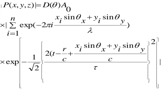
(2.5) Here,  is the pulse width (half) and A0 is the initial sound pressure. The sound pressure at point P(x, y, z) is calculated using the Eq. (2.6) as follows

ri ri i e i c

r t e

n A

i D i z

y x

P  

 

2 }2

) / ( {2 2 1 ) 0

1 ( )

, , (

 



 

(2.6) Here, c is the wave velocity and  is the wave length. If point P is sufficiently far from the center of the UTA then Eq. (2.6) can be expressed as Eq. (2.7) and (2.8) as follows



























































 



 





 







sin 2 sin

( 2 2 exp 1

) 1

sin sin

2 exp(

2 ) 0

( )

, , (











 

 



c

y yi

x xi

c t r n

i

y yi

x xi

i

r i r A e

D z

y x P

(2.7)

The sound pressure becomes as follows

31

| sin 2

sin (

2 2 exp 1

) 1

sin sin

2 exp(

|

) 0 (

| ) , , (

|

































































 



 

 















 



c

y y i

x x i

c t r n

i

y y i

x x i

i A D

z y x P

(2.8)

Here, r is the distance between center of the array O (0, 0, 0) and observation point P(x, y, z). The x and y are the angles of vector OP along with X axis and Y axis, respectively. The wave velocity, wave length and pulse width are denoted by c,  and,  respectively.

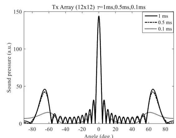
Fig. 2.7 shows the directivity using 1 ms, 0.5 ms and 0.1 ms according to Eq.

(2.8) for time⁡ 𝑡 = 𝑟 𝑐⁄ . The directivity does not change when the pulse width is 0.5 ms, whereas it changes significantly when the pulse width is 0.1 ms.

This is because different elements have different arrival times due to their different distances 𝑟_𝑖. Since the transmitter on the edge of the array is located 55 mm from the center, the maximum difference in the arrival times of different elements is given by Eq. (2.9)

∆𝑡 =

2𝑐

⁡ ⁡

(2.9)

Here, d the inter element space, c the wave velocity and n the number of arrays. The maximum value is obtained 0.16 ms. If the pulse width is shorter than the maximum obtained value by Eq. (2.9), pulse modulation will greatly affect the directivity. However, the main lobe does not change even when the

32

pulse width is 0.1 ms. It is because on the z axis 𝜃_𝑥 = 𝜃, 𝜃_𝑦 = 0⁡ and therefore⁡ ⁡ sin 𝜃_𝑥𝑥_𝑖 + sin 𝜃_𝑦𝑦_𝑖 = 0.

Fig. 2.7: Simulation directivity of ultrasonic transmitter array by modulated pulses 1, 0.5, and 0.1 ms. The sound pressure is normalized by 𝐴₀⁄𝑟.

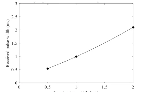
Fig. 2.8 shows waveforms of modulated signals for various directions. The time of origin 𝑡 = 𝑟 𝑐⁄ . The sound pressures are normalized by those obtained using Eq. (2.3) for the continuous wave. The pulse waveform does not change significantly when the pulse width is 1 ms. However, the waveform is significantly affected by the pulse width 0.1 ms but it does not change in the =0^o direction. In time domain, the waveform separates into two peaks increasing the angular direction. It is due to the center of the waveform risen and two pulses eventually merge into a single pulse. The width of the waveform increases with an increase in angular direction.

33

(a) Pulse width: 1 ms

(b) Pulse width: 0.1 ms

Fig. 2.8: Waveforms of modulated signal. The origin of time is 𝑡 = 𝑟 𝑐⁄ . The sound pressure is normalized by Eq. 2.3 for a continuous wave.

-3 -2 -1 0 1 2 3

0 0.5 1

1.5 Directivity(Array 12x12) =1ms =0,20,40,65deg.

Time (ms)

Sound pressure (a.u.)

-0.2 -0.1 0 0.1 0.2 0.3

0 0.5 1

1.5 Directivity(Array 12x12) =0.1ms =0,20,40,47,65deg.

Time (ms)

Sound pressure (a.u.)

0°

20°

40°

65°

0°

20° 40°

65°

47°