File Information Type Doc URL DOI Issue Date Citation Author(s) Title

Instructions for use

Title

Author(s)

Citation

Issue Date

DOI

Doc URL

Type

File Information

THREE ESSAYS ON CULTURAL GOODS TRADE AND DYADIC DATA ANALYSIS

by Yuki Takara

A DISSERTATION Submitted to Hokkaido University

Graduate School of Economics and Business Administration

in Partial Fulfillment of the Requirements for the Degree of

Doctor of Philosophy

June 2018

Copyright c ⃝ 2018 by Yuki Takara

All Rights Reserved

ACKNOWLEDGEMENTS

First and foremost, I would like to show my greatest appreciation to my supervisor, Pro- fessor Shingo Takagi at Hokkaido University, for his insightful comments, suggestions and, especially, teaching of econometrics and programming technique.

I would also like to express my gratitude to dissertation committee members, Pro- fessor Hisamitsu Saito and Professor Nobuhito Suga at Hokkaido University, for their constructive and valuable comments on this dissertation.

My heartfelt appreciation goes to Professor Toshihiro Ichida at Waseda University, for his sophisticated economics lecture at undergraduate school.

I want to thank Professor Hitoshi Inoue and Professor Naoshi Doi at Sapporo Gakuin University and Takahiro Tsujimoto at Tsukuba University, for the invitation to the work- shops and financial supports of trip.

Besides, I would like to offer my special thanks to the faculty members, the staffs and my colleagues at Hokkaido University.

Finally, I would like to send my special thanks to my family, especially to my dearest

grandfather, for the encouragement.

Contents

Contents iii

List of Tables v

List of Figures vi

1 Introduction 1

2 Do Cultural Differences Affect the Trade of Cultural Goods? – A Study in Trade of

Music 7

2.1 Introduction . . . . 7

2.2 Cultural Differences . . . . 10

2.3 Model . . . . 13

2.4 Data . . . . 17

2.5 Result . . . . 21

2.6 Conclusion . . . . 25

2.7 Appendix . . . . 28

3 A Bias Correction Method of Two-Step Estimator for Panel Data Sample Selection Model with Two-Way Fixed Effects 40 3.1 Introduction . . . . 40

3.2 Model . . . . 41

3.3 Bias correction . . . . 44

3.4 Monte Carlo experiments . . . . 49

3.5 Conclusions . . . . 52

4 Measuring the Asymmetric Effects of Cultural Relations on Music Trade Using a Sample Selection Model with Additive and Interactive Fixed Effects 55 4.1 Introduction . . . . 55

4.2 Asymmetry in Cultural Goods Trade Data . . . . 59

4.3 Estimation Procedure . . . . 65

4.4 Estimation Results . . . . 69

4.4.1 Interpretation of Additive Fixed Effect Parameters . . . . 70

4.4.2 Interpretation of Interactive Fixed Effect Parameters . . . . 71

4.4.3 Parameter Estimates . . . . 75 4.5 Conclusions . . . . 77

5 Conclusions 94

Bibliography 97

List of Tables

2.1 Ethnomusicology Based Classification . . . . 30

2.2 Civilization Based Classification . . . . 33

2.3 Country List . . . . 35

2.4 Definition of Variables . . . . 36

2.5 Summary Statistics (full sample) . . . . 36

2.6 Summary Statistics (Latin–Western) . . . . 37

2.7 Summary Statistics (Asian) . . . . 37

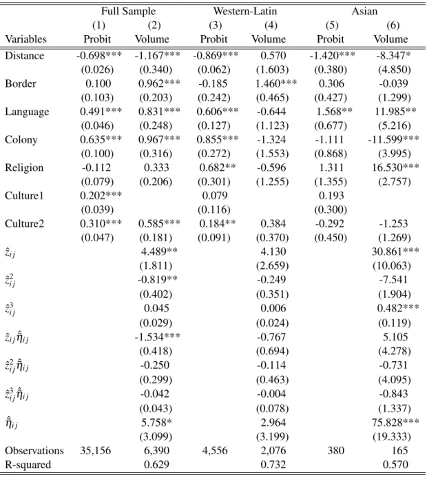
2.8 Estimation Results . . . . 38

2.9 Check the Validity of Excluded Variable . . . . 39

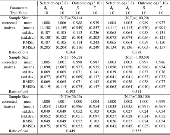
3.1 Simulation Result: Sample Selection Model with Static Selection Equation . . 53

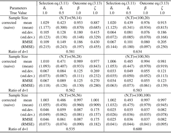
3.2 Simulation Result: Sample Selection Model with State-dependent Selection Equa- tion . . . . 54

4.1 Country List . . . . 82

4.2 Definition of Explanatory Variables . . . . 83

4.3 Summary Statistics . . . . 83

4.4 Asymmetric Country Pairs . . . . 84

4.5 Symmetric Country Pairs . . . . 85

4.6 Contribution Ratio of Each Factor in Outcome Equation . . . . 85

4.7 Regression results of cultural variables on estimated interactive effects in the selection equation . . . . 88

4.8 Regression results of cultural variables on estimated interactive effects in the outcome equation . . . . 88

4.9 Estimation Result: Selection Equation (4.1) . . . . 91

4.10 Estimation Result: Outcome Equation (4.2) . . . . 91

List of Figures

4.1 Additive Fixed Effects of the Outcome Equation on the World Map . . . . 86

4.2 Additive Fixed Effects of the Selection Equation on the World Map . . . . 87

4.3 First Interactive Terms of the Outcome Equation on the World Map . . . . 89

4.4 Second Interactive Terms of the Outcome Equation on the World Map . . . . . 90

4.5 Third Interactive Terms of the Outcome Equation on the World Map . . . . 92

4.6 Forth Interactive Terms of the Outcome Equation on the World Map . . . . 93

Chapter 1

Introduction

In the field of economics, culture and art have been discussed long before the term “Cultural Economics” was coined in the twentieth century. The accumulated research findings are summa- rized in the “Handbook of the Economics of Art and Culture” (Ginsburgh and Throsby (2006)), which covers the broader topics of economic problems related to art and culture. Economists have addressed economic problems related to cultural topics, for example, “positive or nega- tive externalities associated with arts,” “an effect of patronages on arts,” “whether a free market achieves supplies of arts at an optimal level or not,” and “the government’s role as a supporter or operator in a market of art” (Goodwin (2006)).

These economic topics related to culture and art have been discussed from the past right

up to the present day. In particular, to deal with the problem of cultural convergence or inva-

sion, the roles of government and international institutions have been discussed by many cultural

economists and cultural institutions such as United Nations Educational, Scientific and Cultural

Organization (UNESCO). The recent development of distribution technologies and communi-

cation tools has led to a reduction in trade costs. As a result, imports from large countries have

increased and influx of foreign culture prevails against their own culture. For example, we can

eat a hamburger, drink a Coke and enjoy Hollywood movies, and American pop music in almost

every country on earth. This type of consumption can be viewed as cultural convergence or as a cultural invasion by economically developed countries.

UNESCO has declared its commitment to protect and promote diversity of cultural expres- sions (the 2005 Convention for the Protection and Promotion of the Diversity of Cultural Ex- pressions, UNESCO (2013)). Economic researchers often discuss the relationship between trade and cultural diversity. Mas-Colell (1999) raised the question of whether or not should we differ- entiate cultural goods from other conventional goods. Using trade data, Ferreira and Waldfogel (2013) confirmed whether there is cultural convergence in the music market or not. They fo- cused on cultural protection polices, such as “airplay quota,” in some countries (for example, Canada, France, Australia, and New Zealand) and analyzed whether the policy could limit the cultural invasions, such as by the U.S., or not. Disdier et al. (2010) use naming data in France and suggest that the audio-visual service trade could transform domestic tastes and cause foreign culture to supersede domestic culture.

While there are some discussions that cultural goods exports from large countries cause cultural convergence, others suggest that exports from a large country do not have an impact on the domestic culture. If cultural differences (or lack of cultural proximity) between two countries act as trade costs, they reduce the export from culturally distant countries. In this case, consumers tend to choose domestic or culturally familiar foreign goods and the prevalence of exports from large countries could not occur as a result (a home consumption bias). One example is export of “Country” music from U.S. to Asian countries. Country music have smaller market share in Asia compared to that in U.S. This could be considered that, because Asian countries do not share the cultural backgrounds of U.S., the market share of country music in Asia is small.

In this case, the difference of cultural backgrounds acts as trade friction cost and inhibits the

export from culturally distant countries.

To summarize, discussions of the cultural convergence or invasions are related not only to economic statuses but also proximity of cultural backgrounds each country has. If cultural prox- imity promote demands for culturally familiar foreign goods, the serious cultural convergence or invasions would not occur and vice versa. Hence, to reveal the role of cultural proximity as a cost in cultural goods trade is an essential work.

A gravity model of trade is suitable to analyze this topic

. The model states that there are mainly two important factors of the cultural goods trade corresponding to the aforementioned discussions. One is the effect of economic conditions such as the gross domestic product (GDP) and the other is the effect of trade friction costs that includes cultural factors. On one hand, it is clear that economic size has substantial influence on the trade of cultural goods. Existing studies show that the size of an economy has a significant effect on cultural goods being traded in the same way as conventional goods (Schulze (1999); Holloway (2014)).

On the other hand, the effect of cultural proximity as trade friction costs on consumers is hard to reveal. Many of the existing empirical studies on trade attempt to control cultural fac- tors using linguistic differences, religious proximity, and past colonial relations. However, they represent not only the cultural proximity but also the other trade friction costs such as negotia- tion costs. Hence, these cultural variables could not be suitable for our research question. For example, a positive estimated coefficient of linguistic proximity could not imply that consumers prefer culturally similar goods, since it represents not only cultural proximity but also the trade negotiation cost of cultural goods. For this reason, we need to consider cultural factors more carefully and introduce cultural variables that represent the proximity itself when discussing the effect of culture on the trade of cultural goods.

Some studies highlight the importance of cultural factors in the trade and introduce novel

1

The gravity models under a monopolistic competition assumption are summarized in Feenstra (2015).

cultural variables that can capture cultural proximity itself. Guiso et al. (2009) introduce bi- lateral trust measures taken from a survey conducted by Eurobarometer as a cultural variable.

Felbermayr and Toubal (2010) use cultural variables based on the Eurovision Song Contest Score and analyze the trade within Europe. Tadesse and White (2010) use the data of Inglehart et al. (2004) and Hagenaars et al. (2003) to calculate the “Cultural Distance” between the two countries. Giuliano et al. (2014) use a “Genetic Differences” index as a proxy of the cultural differences index.

One common way to create a cultural variable is to use the World Values Survey

, the most well-known and popular survey related to social sciences (including cultural studies). The survey is conducted globally and provides a rich insight into people’s beliefs, values, and information.

Noteworthy characteristics of this survey are that the raw results of questionnaires are available and we can extract some feature values that represent people’s values by using methods of mul- tivariate analysis such as Principal Component Analysis (PCA). However, we need to be careful when using the aforementioned data, since it is hard to decide whether the value represents the cultural factors that we intend to capture. The term “culture” is an ambiguous concept; culture is made up of linguistic factors, religious concepts, differences in values, nationality, humanity, history, and many other factors. It is necessary to specify what the value captures when we use the World Values Survey data.

The other way to create a cultural variable, we demonstrate in this dissertation, is to use interview-based studies as a source of data. Although this restricts the research subject to one specific cultural good, the cultural variables that are based on such studies can adequately cap- ture cultural factors. For example, our cultural variable based on an ethnomusicological study (Lomax (1959)

) can capture cultural factors in the context of music. The ambiguous definition

2

The World Values Survey is one of the largest, repeated cross-section survey. The data and the documentations are available at:

3

Some researches raise critical comments on this study (for examples, Driver and Downey (1970), Nettl (1970)).

of culture occurs when we treat cultural goods as one category. We can define culture in the context of movies, music, paintings, or novels if only we focus on these goods.

In addition, we propose a novel method to extract cultural factors from the data of traded cultural goods. Cultural factors can be thought of as country-specific, as each country has its own culture. When countries trade, we can control the effects of such cultural factors with additive fixed effects if one cultural factor (for example, the exporting country’s culture) is independent of the other one (importing country’s culture). However, this is not necessarily the case. For example, Japanese culture may be preferred by one country but disliked by another. In this case, Japanese culture is Japan-specific, but the effects depend on the partner country. We consider that the effect of country-specific culture that affects the trade of cultural goods depends on the partner country, and we call this the “cultural relations.”

Cultural relations are represented in the empirical model as interactive fixed-effect terms.

Following the estimation procedure of Bai (2009), we can identify the values of interactive terms. It should be noted that we should carefully discuss whether the values of interactive terms represent the cultural relations, since our estimation procedure is similar to the PCA. While our estimated value of interactive terms contains information on cultural relations, it also contains information on other relations, for example, spatial correlations. Nevertheless, our approach toward the cultural relationship is noteworthy. This type of approach extends the knowledge of cultural studies in the field of cultural economics, especially in the trade of cultural goods.

To summarize, the main purpose of this dissertation is to reveal the relations between cultural factors and trade of cultural goods. First, we show the impact of cultural proximities (or differ- ences) on the trade of cultural goods, using cultural variables that are based on other cultural studies. We then extract the cultural relations from the data of cultural goods traded, controlling

Recent studies (for examples, Panteli et al. (2017), Gold et al. (2017)) shed new light on Lomax (1959)’s attempts

using machine-learning and other computerized technologies of analyzing music data.

the other economic factors that are used in many existing studies of trade. Through this disser-

tation, we employ the gravity model of trade proposed in Helpman et al. (2008). Our approach

toward the cultural factors and trade of cultural goods is novel and sheds some light on the role

of cultural factors in cultural economics. This dissertation consists of five chapters. Chapter 1 is

the introduction. In Chapter 2, we show the empirical result of the effect of cultural differences

on the trade of cultural goods. In Chapter 3, we discuss the analytical bias correction method

used in Chapter2, that is incidental to the panel data analysis with two-way fixed effects. We

extend the concept of cultural differences to cultural relations and show the estimated result of

the cultural relations in Chapter 4 and Chapter 5 concludes the dissertation.

Chapter 2

Do Cultural Differences Affect the

Trade of Cultural Goods? – A Study in Trade of Music

2.1 Introduction

In recent years, music has become one of the most valuable items in the trade of cultural goods

1

. A report by UNESCO (2016) shows that the export share of recorded sound media was the second largest in the trade of cultural good from 2004 to 2013. Cameron (2015) points out that owing to the recent technological progress in media recording and broadcasting through the internet, music became a “highly global economic phenomenon.” Music producers can produce and immediately release songs worldwide. Consumers can access information about their favorite artist and even buy his/her songs despite the geographical distance. However, even though the progress of the globalization of music industry was expected to promote the trade of music, from 2000 to 2006 only 18% of trade paths traded music compact discs (CDs), whereas 65% of trade paths were active in terms of total goods trade.

Standard trade theory predicts that trade volume is determined by cost, productivity, factor

1

UNESCO (2009) defines cultural good : “Consumer goods that convey ideas, symbols and ways of life, i.e.

books, magazines, multimedia products, software, recordings, films, videos, audio–visual programmes, crafts and

fashion.”

endowment, etc.. In the case of cultural goods, including music, we also consider “cultural differences” as important determinants of trade volumes; however, the relationship between the trade of cultural goods and cultural differences is unclear. The purpose of this study is to define cultural differences and to assess whether such differences affect the trade of cultural goods.

To this end, we use a large dataset of traded music CDs and the gravity model of trade. While Felbermayr and Toubal (2010) and Holloway (2014) investigate the relation between the trade of cultural goods and cultural differences using a gravity type model, this kind of approach to the cultural good trade is relatively rare.

When analyzing the international trade, we address the existence of the zero–trade path, which causes a sample selection bias. In addition, we discuss the omitted variable bias that may arise due to the lack of producers’ “productivity” data. To avoid these biases, we use the gravity model of trade proposed by Helpman et al. (2008). This model can correct the sample selection bias and control the effect of latent music “productivity,” which can differ across countries. We disentangle the effect of cultural differences, using this type of gravity model to control the observable and unobservable determinants of trade.

Among the determining factors of trade appearing in usual gravity models, costs are the most important factor. In general, there are two kinds of trade costs: “transportation” cost as variable one and “entry” cost as fixed one. In the gravity model by Helpman et al. (2008), the trans- portation costs appear in both the selection and outcome equations, while the entry costs appear only in the selection equation

. In empirical studies, the transportation costs are represented as “distance between two countries” or “contiguousness dummy.” The entry costs, on the other hand, are represented as “common language dummy,” “religious proximity,” or “FTA dummy

3

.” When we analyze the total trade volume, these variables correctly represent the transporta-

2

In Helpman et al.’s (2008) gravity model, countries firstly decide either to start trading or not (the first-stage selection equation), and then decide how much they trade (the second-stage outcome equation).

3

Cultural variables are often used as measurements of entry costs.

tion and entry costs. Helpman et al. (2008) show that the distance between two countries has significant effects on both the probability of trade occurrence and the volume traded. This result implies that “distance” is a good measurement of transportation costs. They also indicate that variables that represent the entry costs have a significant effect on the probability of trade occur- rence, but have no significant effect on trade volume. This implies that these variables are good measurements of entry costs.

However, when analyzing the cultural goods trade, this is not the case. Ferreira and Wald- fogel (2013) analyze the trade of music using a gravity equation and show that the language dummy has significant effects on both the probability of trade occurrence and volume of music traded. If the language dummy represents the entry cost of trade, this variable might have a significant effect only on the probability of trade occurrence. From the estimation result, we can conclude that the language dummy does not indicate the entry cost in the case of cultural goods trade. Rather, we can consider that the language dummy indicates a variable cost of music trade.

This consideration does not seem exaggerated. Considering lyrics, if a destination uses the same language as the origin, consumers can better understand the intent of the lyrics. Therefore, the language dummy has a significant positive effect on the music trade volume. Hence, we presume that the variables that seemed to indicate entry costs in previous studies indicate a variable cost when analyzing the trade of cultural goods, including music.

Regarding the costs, “cultural differences” must be considered in addition to the usual ex- planatory variables. We assume that some kind of cultural difference exists between two coun- tries, and the differences affect the choice of consumers. “Country music” is a good example.

“Country music” is very popular in the United States

and in those countries that share the American culture, such as Canada and Australia. However, in countries that do not share the

4

The share of country music in the United States was about 15% in 2014. This is the third largest share.

Source:2014 Nielsen Music Report

(http://www.billboard.com/articles/business/6436399/nielsen-music-soundscan-

2014-taylor-swift-republic-records-streaming?page=0%2C3)

American culture, this is not the case. Indeed, in the Asian region, country music is not a popu- lar music genre

. Thus, it is natural to consider the cultural differences as trade cost.

The purpose of our study is to find cultural variables that capture the cultural differences and to reveal the relation between trade behaviors and cultural differences, supported by sound econometric method. An important and difficult aspect of our study is how to classify culture.

We analyze only the trade of music as a representative of cultural goods; therefore, we can define the cultural differences in the context of musical culture. We find that country pairs that share the same culture tend to trade significantly more compared to the country pairs that do not. Moreover, one of our cultural variables helps us to satisfy the exclusion restriction of the two-stage estimation procedure.

This study is organized as follows. In section 2.2, we highlight the definition of cultural differences and its measurement method. In section 2.3, we introduce the gravity model of international trade and explain the parameter estimation technique. In section 2.4, we describe the data used for our analysis. In section 2.5, we show the estimation results, and section 2.6 concludes.

2.2 Cultural Differences

Here, we provide the definition of cultural difference and its measurement. Cultural differ- ences are important determinants of trade volume that affect the consumer choice. However, only a few studies have examined the cultural differences because an accurate quantification of the differences in culture is difficult. In studies such as by Guiso et al. (2009), Disdier et al.

(2010), Felbermayr and Toubal (2010), Tadesse and White (2010), Gokmen (2012), Giuliano et al. (2014), and Holloway (2014), they have attempted to capture the cultural difference and

5

For example, Garth Brooks, one of the most successful country musicians, who charted in Billboard 200 in 2014,

did not chart in Billboard Japan Hot Overseas chart in 2014.

perform analysis using cultural variables defined therein. In our study, we focus only on the music trade to capture the cultural difference correctly. Owing to this limitation of the subject of research, we can define the cultural difference in the context of music.

However, before defining the cultural difference, let us explain a cultural region, which is a basic concept when discussing cultural differences. As with other phenomena with broad classifications, we assume that culture can also be classified into several groups. Here, we call the cultural groups as “cultural regions”, and define cultural difference as follows: If two countries are not in the same cultural region, there is a cultural difference between the two countries. Using this definition, we can deal with cultural differences if we classify the countries into several cultural regions.

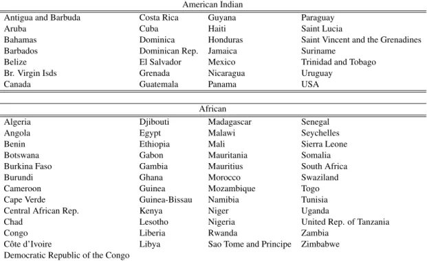
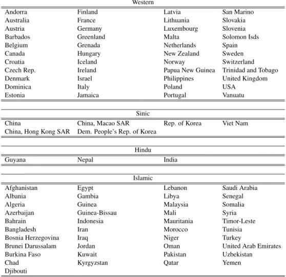
The question is how to classify the various regions. Here, we consider two comprehen- sive and intuitive ways of classification: “ethnomusicology-based classification” by Lomax (1959) and “civilization-based classification” by Huntington (1996). Lomax (1959) uses the ethnomusicology-based classification to classify all musical styles into ten styles: American Indian, Pygmoid

, African, Australian, Melanesian, Polynesian, Malayan, Eurasian, Old Eu- ropean, and Modern European. This comprehensive classification explains the differences such as the melody structure, performance method, and social and religious meaning

. This clas- sification captures the musical difference across cultures. We define these regions as “musical region” in this study. Huntington (1996) uses the civilization-based classification to categorize all countries into eleven regions: Western, Sinic, Islamic, Hindu, Orthodox, Latin American, African, Buddhist, Japan, Haiti, and Ethiopia. We consider that this classification captures the difference of mass culture. We define these regions as “civilization region” in this study. The lists of countries and corresponding classification of cultural regions are reported in Table 2.1

6

We do not consider the Pygmoid region, as it is difficult to identify the countries that constitute this region.

7

Note that, following this classification, some countries belong to two or three musical regions. For example,

France and Spain belong to Eurasian, Old European, and Modern European regions.

and 2.2.

Using these classifications, we define two cultural dummy variables: Culture1 and Culture2.

If an origin and a destination country are in the same musical region, the Culture1 dummy takes a value equal to 1, and 0 otherwise. This variable represents the cultural proximity (or lack of difference) in terms of traditional meaning. If two countries share the traditional music culture, Culture1 takes a value equal to 1. Similarly, if both countries are in the same civilization region, the Culture2 dummy takes a value equal to 1, and 0 otherwise. This variable represents the cultural proximity (or lack of difference) in terms of modish meaning. If two countries share the modern cultural attitude, Culture2 takes a value equal to 1. For example, consider the case of Egypt and Italy. Egypt and Italy are in the same “Eurasian” musical region; hence, Culture1 takes a value equal to 1 for Egypt–Italy and Italy–Egypt trade paths. On the other hand, Egypt is in the “Islamic” civilization cultural region and Italy is in the “Western” civilization cultural region; hence, Culture2 takes a value equal to 0. Both Culture1 and Culture2 take a value equal to 1 if two countries share the corresponding culture, and 0 otherwise. The corresponding estimated coefficients become positive if our hypothesis is true.

In addition, we assume that there are two types of consumers: “devotee” and “mass” con-

sumers. We define devotees as consumers who are keen on music. Since they are enthusiastic

music consumers, they are sensitive to the musical and mass cultural differences, seek music

from around the world and introduce it to their own country’s market. On the other hand, we de-

fine masses as consumers who are not keen on music compared to devotees. Therefore, they do

not pay a particular attention to the musical cultural differences and are only concerned with the

mass cultural differences. From these definitions, we infer that devotees can be affected by Cul-

ture1 and Culture2 because Culture1 captures the musical cultural proximity (or difference) and

Culture2 captures the mass cultural proximity. On the other hand, masses can be only affected

by Culture2 because they do not focus on the musical cultural differences, which are captured by Culture1. In addition, we also assume that the number of mass consumers is larger compared to devotees. This assumptions does not seem to be arbitrary, as most music consumers behave as masses rather than devotees, while only a few enthusiastic music consumers act as devotees.

These are essential assumptions of our study and help us estimate the gravity equation. We will explain the importance of these assumptions in the next section.

2.3 Model

Here, we introduce the gravity model we used in this paper, which follows Helpman et al. (2008)

8

. To summarize, the model explains why some countries trade and others do not from the perspective of productivity heterogeneity. In this model, suppose that a producer-specific pro- ductivity a is distributed and can be described by a cumulative distribution function G(a) with support [a

, a

]. In the case of cultural goods trade, “producer” corresponds to the artist (in the case of music trade, a singer or a band) and producer-specific productivity can be considered as an ability to make arts (e.g., Ferreira and Waldfogel (2013)).

Besides, we should pay attention to what represents the fixed cost of trade in the music trade. In the case of total trade, regulation cost of a firm entry, measured by the number of days and/or legal procedures, expresses the fixed cost of trade (e.g., Helpman et al. (2008)). These measurements affect the decision of trade entry but have no effect on trade volume. In the case of music trade, the entry cost of artists to participate in the foreign market (a kind of notification cost, which is required for artists to be recognized by consumers in foreign countries) could express the fixed cost. A part of such cost is measured by traditional relation of two countries in the context of music. If two countries are traditionally related, artists might enter the market in

8

Most of the symbols that we use for variables correspond to those used by Helpman et al. (2008).

partner country at low cost.

In this study, the traditional cultural variable Culture1 is good measurement of this fixed cost. On the other hand, as discussed in section 2.1, linguistic proximity, past colonial relations, religious proximity and modern cultural variable Culture2 could be measurements of variable cost.

Consider a variable that represents the proportion of profit for the most productive producer to the common fixed cost to export:

Z

≡ (1 − α ) (

Ti jcj

)

Y

a

c

f

, (2.1)

where Y

is the income of country i, P

is the price index in country i, ε is the elasticity of substitution across goods, α is the parameter that fulfills 0 < α < 1, and T

, c

, f

represent the cost factors. T

express the variable costs including transportation costs; T

> 1 for all i ̸ = j and T

= 1 for all trade within country j. c

f

express the fixed costs; c

is country specific and f

is trade path i-j specific and f

> 0 for all trade paths i ̸ = j. We assume that the trade path i-j specific cost f

is stochastic. Let f

≡ exp( ϕ

+ ϕ

+ κϕ

− ι

), where ι

is an error term and ι

∼ N(0, σ

), ϕ

is is the fixed export cost common across all export destinations, ϕ

is a fixed trade barrier, and ϕ

is a country-pair-specific observed fixed cost. Then, we assume that T

is also stochastic because there is unmeasured trade friction u

. We define T

≡ D

e

, where D

is the observed index of variable costs between country i and j, such as distance between two countries, and u

∼ N(0, σ

). The positive export from country j to i is observed only if Z

> 1.

Using these specifications, the logarithm of the variable Z

is

z

= α

+ λ

+ χ

− γ d

− κϕ

+ η

, (2.2)

where η

≡ u

+ ι

∼ N(0, σ

+ σ

), λ

and χ

represent the exporter and importer fixed effects, respectively (these contain the information of price index, income, importer/exporter fixed costs, etc.). The lowercase letters refer to the natural logarithm of their uppercase variables.

Then, assume that as σ

+ σ

= 1, the probability that country j exports to country i condi- tional on observed variables can be expressed as

ρ

= Pr(I

= 1 | ObservedVariables)

= Φ ( α

+ λ

+ χ

− γ d

− κϕ

), (2.3)

where I

is the indicator function that takes a value equal to 1 if country j exports to country i and 0 otherwise, and Φ ( · ) is the cumulative distribution function of standard normal distribution.

Equation (2.3) estimates the probability that country j starts to export music to country i. It is not possible to observe z

, but we can calculate the value of z

using equation (2.3). We call equation (2.3) the first-stage selection equation.

Then, consider the volume of trade. The trade volume from country j to country i is ex- pressed as

M

= ( T

c

α P

)

Y

N

V

, (2.4)

where N

is the number of goods that are available in country j, and V

indicates the fraction of exporting producers. Suppose that the productivity 1/a follows a truncated Pareto distribution, and this assumption indicates that we can rewrite the expression as

V

= θ W

, where W

= max (( a

a

)

− 1, 0 )

, (2.5)

where θ is a constant parameter and k is the shape parameter of the truncated Pareto distribution.

Equation (2.4) can be expressed in a log-linear form as

m

= β

+ λ

+ χ

− γ d

+ w

+ u

, (2.6)

where β

is a constant term, and λ

and χ

represent the exporter and importer fixed effects, respectively (these contain the information of price index, income, population, etc.). The lower- case letters refer to the natural logarithm of their uppercase variables.

To estimate the consistent estimator, we need to control the endogenous effect of the number of exporters, w

, and the selection bias. Taking conditional expectations, equation (2.6) can be rewritten as

m

= β

+ λ

+ χ

− γ d

+ h(ˆ z

, η ˆ¯

) + β

η ˆ¯

+ e

(2.7) where ˆ¯ η

= ϕ (z

)/Φ(z

), ϕ (·) is probability density function of standard normal distribution, ˆ

z

= Φ

( ρ ˆ

), h( z ˆ

, η ˆ¯

) is the third polynomial function

of ˆ z

, and ˆ¯ η

, β

= corr(u

, η

)( σ

/ σ

), corr(a, b) is a correlation coefficient between a and b, and e

is an error term with e

∼ N(0, σ

).

We call equation (2.7) the second-stage outcome equation.

To summarize the estimation model, we use equations (2.3) and (2.7). First, we estimate equation (2.3) and calculate the values of ˆ z

(estimated value of z

, the unobserved ratio of the export profit to the fixed costs) and ˆ¯ η

(inverse Mills ratio, which corrects the sample selection bias) using the estimation result. Then, we estimate equation (2.7).

When we estimate the outcome equation, we need to exclude at least one variable from the equation, which does not appear in outcome equation such as observed fixed costs ϕ

. The choice of the variable that we exclude is crucial. The estimated coefficients and their variances

9w_{i j}

is a concave function and have lower bias if we directly take an expectation. To avoid this bias, we first

approximate

with a polynomial in ˆ

and ˆ¯

, and then, we take an expectation of

. The value is described as

1] =

ˆ

ˆ

ˆ

ˆ¯

ˆ

ˆ

ˆ

ˆ¯

will be significantly biased if we exclude an inappropriate one

.

In our study, the variable Culture1 can be viewed as the observed fixed cost ϕ

. From our assumption of devotees and masses in section 2.2, we suppose that Culture1 affects only devotees and the number of devotees is small. In the case that Culture1 equals to 1, devotees tend to import music from its trading partner compared to the case that Culture1 equals to 0. However, once two countries start trade, the volume of music traded does not depend on Culture1 since Culture1 affects only devotees and the number of devotees is extremely smaller compared to masses. Culture1 reduces the trade starting cost through the act of devotees but has no effect on trade volume. Thus, Culture1 can be considered as fixed cost ϕ

in the model.

On the other hand, the variable Culture2 can be viewed as the variable cost d

. If Culture2 equals to 1, devotees and masses tend to import music from the trading partner. Recalling that the number of masses is larger in the market, the volume of music traded is promoted in the case that Culture2 equals to 1. Therefore, Culture2 can act as the variable cost d

in the model.

After estimating the parameters, we perform an additional bias correction. Panel data mod- els using fixed effects can cause incidental parameter problem and the parameters become biased severely when the model is nonlinear. To correct this bias, we use the bias correction method proposed by Fern´andez-Val and Weidner (2016) and expand it to apply to our two-stage estima- tion model. The details of these correction methods are in appendix 2.7.

2.4 Data

We use the amount of traded CDs as a proxy of the traded music. The data employed in this study are from 2000 to 2006 and cover 188 countries. The list of these countries is provided

10

In Helpman et al. (2008), they assume religious proximity as excluded variable in their dataset. Following this,

Ferreira and Waldfogel (2013) also exclude the religious variable. However, we need to be more careful on the choice

of excluded variable.

in Table 2.3. The trade data of music is from the United Nations Commodity Trade Statistics Database (http://comtrade.un.org/), which is the most comprehensive database

. We use an HS Code classification that is popular and detailed one. The commodity code is HS8524.32: discs for laser reading systems for reproducing sound only.

As we calculate an average value from 2000 to 2006 to avoid a year–specific effect, our dataset is essentially cross–sectional. The variables of our data contain two indexes, for importer i and exporter j, and the data can be arranged as if they were an N × N panel dataset

. The most significant difference between a general panel dataset and our data is that the diagonal elements M

(exports from some country j to the country j) are always omitted by definition. In addition, the trade data is asymmetric, that is, M

(export from a county j to a country i) need not be equal to M

(export from a county i to a country j), although some explanatory variables must be symmetric (for example, Distance

= Distance

).

The explanatory variables are geographic distance, common border dummy, common lan- guage dummy, colonial tie dummy, religious proximity and two cultural proximity dummies (Culture1 and Culture2). These variables except Culture1 represent the variable cost of trade and are included in the variable cost d

in the estimation model. On the other hand, as afore- mentioned in section 2.3, Culture1 would represent the fixed cost and are included in ϕ

in the selection equation. The data for geographic distance, common border dummy, common lan- guage dummy and colonial tie dummy were obtained from the Centre d’ ´ Etudes Prospectives et d’Informations Internationales (http://www.cepii.fr/) database. The religious proximity variable is calculated in the same way as in Helpman et al. (2008), using the dataset introduced by Alesina et al. (2003). We also use the cultural dummy variables introduced in the previous section. The

11

Other databases that provide trade data include NEBR-UN and CHELEM. However, Comtrade provides a higher level of sector disaggregation (6-digit) and covers a rather unlimited number of countries (Gaulier and Zignago, 2010).

12

In this case, the row index assign to importer countries and the column index assign to exporter countries.

definitions of independent and dependent variables are provided in Table 2.4.

When using data of music traded, we need to take into account the effects of intellectual property right (IPR) protection levels (for example, IPRI (2017) and World Economic Forum (2017) provide such data respectively) on the trade volume. Shin et al. (2016) show that the IPR protection levels of the importing country have positive effect on total trade value. On the other hand, Aguiar and Waldfogel (2014) point out that copyright protection reduces the consumption choice of music in the foreign market. However, in either case, such country specific institutional effects can be controlled by country–specific fixed effect terms in our model, since the IPR protection levels of importing or exporting country are country–specific.

In addition, we need to consider how to treat the effects of digital piracy on the sales.

There are many studies about the relationship between piracy and cultural goods sales (e.g., Oberholzer-Gee and Strumpf (2007); Rob and Waldfogel (2006); Zentner (2005)). However, the effect of piracy rate on the music sales is still unclear; moreover, there has been no con- clusive theories or empirical studies. In this study, we consider that the effect of piracy on the volume of music traded is negligible. Oberholzer-Gee and Strumpf (2007) show that, in 2003, most of file sharing users were in large countries, such as the United States (30.9%), Germany (13.5%), Italy (11.1%), and Japan (8.4%)

. Aside from these large countries, this fact allows us that it is possible to ignore the effect of piracy on the music traded in small countries that occupy the major part of our sample. In large countries that have many file-sharing-software users, there is a possibility that the trade volume data reported from such large countries are smaller than the actual traded volume owing to the effect of illegal downloads. However, we can also avoid this possibility. Rob and Waldfogel (2006) state that the willingness to pay for music that is downloaded illegally is lower than music purchased. This implies that the sales of CDs

13

The number of file sharing users in top 16 countries was about 93% in 2003.

do not depend on whether there is piracy, because the music download illegally would not be worth paying money. As mentioned above, we consider that the piracy does not affect the sales or trade volume of music regardless of countries size.

Similarly, the effect of digital content sales must be taken into consideration. Digital music became more significant in the current music industry; however, tracing the trade flow of digital contents is extremely difficult. The purpose of this study is to reveal the impact of cultural differences on music trade. For this purpose, comparing physical and digital music, physical contents seem desirable because they are traceable and widely traded around the world compared to digital contents

. In our sample period, we can confirm that digital media have negligible effects on trade. Based on the IFPI (2012) report, the market share of digital music is small

in our sample and is mainly concentrated in the United States and Canada. Furthermore, in our sample period, digital contents were not available in many countries

. This implies that there should not be an underestimation of the trade volume, which is caused by digital music sales, in almost all trade paths. Therefore, we conclude that the digital media do not have a significant impact on our estimation result and conclusions

.

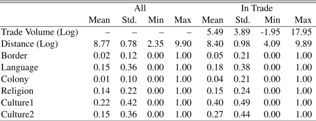
Column “All” in Table 2.5 shows the summary statistics of dependent and independent vari- ables. From the table, only 2% of the country pairs share a border. The ratio of country pairs sharing a language is 15% and country pairs that were in a colonial relation are only 1%. The average religious proximity is 0.14. Of the country pairs, 22% are in the same music cultural region and 15% share the mass culture. Column “In Trade” in Table 2.5 shows the summary

14

Moreover, IFPI (2015) reports that in 2014 physical music contents had 46% share, which is equivalent to the digital ones. Therefore, physical goods data do not seem to be outdated for investigating cultural trade.

15

The global share of digital music was 0% from 2000 to 2003, 2% in 2004, 5% in 2005, and 10% in 2006.

16

For example, iTunes Store, which is the pioneer of music download service, started their service in 2003 and had provided the service for only four countries in July 2004, and twenty countries in August 2006.

(http://www.apple.com/pr/).

17

Of course we should consider the digital music contents data if it is traceable. This is the further research topic

of this study.

statistics only for country pairs that have traded at least one unit of music. Compared to the full sample summary, the mean values of all variables, except Distance, increase. For positive trade flows, 40% of the country pairs are in the same music cultural region, and about 27% of the country pairs are in the same mass cultural region. From this summary, it can be expected that, as the value of these variables increase, they will have a positive effect on the probability ρ

.

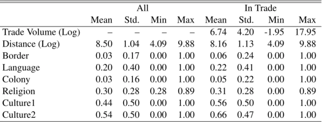
In addition to the full sample, we prepare subsamples for advanced analysis. We use “Western- Latin” sample and “Asian” sample. Columns “All” and “In Trade” in Table 2.6 respectively show the summary statistics of the Western-Latin sample and Western-Latin sample of only for the country pairs that have traded at least one unit of music. In the Western-Latin sample, the degree of cultural proximity is high compared to the full sample. Columns “All” and “In Trade”

in Table 2.7 respectively show the summary statistics of Asian sample and Asian sample of only for country pairs that have traded at least one unit of music. In the Asian region, the degree of mass culture proximity is low, although the degree of musical culture proximity is high. These tendencies are in common with all samples and samples with positive trade.

2.5 Result

Table 2.8 reports our estimation results. Columns (1) and (2) in Table 2.8 show the estimation result using full sample. Column (1) shows the estimates of the selection equation, and column (2) represents the estimates of the gravity equation with endogeneity controlling variables. In column (2), we use only positive trade flow.

In column (1), all variables except Border and Religion have significant effects on ρ

. As

standard gravity estimates indicate, the distance between two countries has a negative effect on

the probability of trade occurrence, ceteris paribus. Similarly, the country pairs using the same

language and were in the colonial ties are likely to start trade significantly more compared to

other country pairs. In addition, the estimation results show that both Culture1 and Culture2 have significant positive effects on ρ

. These results support our hypothesis that consumers are likely to choose a trading partner that culturally resembles each other.

Column (2) shows the estimation result of the outcome equation. To estimate this equation,

we use Culture1 as the excluded variable. As we stated in the previous section, we consider

that Culture1 has no effect on masses; therefore, Culture1 has a significant effect on ρ

and

non-significant effect on the volume of music traded. Hence, this variable can be excluded to

satisfy the exclusion restriction. In addition, we introduce endogeneity controlling variables,

their polynomial terms, and cross terms in the second-stage estimation. Similar with the Probit

estimation results in the first stage, all variables except Religion has a significant effect on music

trade volume, while Distance has a negative effect on the trade volume. The variables Border,

Language, and Colony have significant positive effects on trade volume. Other things being

equal, a pair of countries trade music about two and a half times (= exp (0.962)) more if they

are contiguous, two times (= exp (0.831)) more if they use the same language, and two and a

half times (= exp (0.967)) more if the countries have colonial ties. The variable Culture2 also

has a significant positive effect on the music trade volume, although the impact on the trade

volume is relatively small compared to border, language, or colonial tie dummies. Other things

being the same, a country exports music about two times (= exp(0.585)) more if both countries

belong to the same cultural region. Thus, we can assert the importance of the effect of cultural

difference on the trade volume. Our intuitive hypothesis that cultural differences affect the

consumer choice, ceteris paribus, is supported by our estimation results. We intuitively know

that when we consume foreign music, we choose the one that is more familiar. However, we

cannot specify whether the choice is a result of the cultural difference or, for example, of the

linguistic difference. After controlling for other conditions, such as language, colonial relation,

income, distance between two countries, etc., our estimation results show that cultural difference significantly affects the consumer choice.

Next, we show the estimation results using the subsamples. Columns (3) and (4) in Table 2.8 show the estimation result using the Western-Latin subsample. In column (3), all variables except Border and Curture1 dummies have significant effects on ρ

. This result is similar to the one in the full sample. The main differences between the full sample result (column (1)) and the Western-Latin subsample result (column (3)) are (a) Religion has a significant effect on ρ

, and (b) Culture1 dummy has no significant effect on ρ

. Within the Western-Latin region, the cultural difference of music does not have a significant effect on the probability of trade occurrence ρ

. Column (4) shows a very different result. Here, only Border dummy has a significant effect on the trade volume. Even the control variables ˆ z

, ˆ¯ η

, and their cross terms that represent the productivity (or export ability) have no significant effects on the trade volume.

Besides, the standard errors of estimated coefficients take larger values. We conclude from this estimation result that we fail to estimate the parameters of outcome equation using the Western- Latin subsample. Within the Western-Latin region, the variable Curture1 does not behave as we expected.

The estimation results using the Asian subsamples are in columns (5) and (6) in Table 2.8.

Column (5) shows that only Distance and Language dummies have significant effects on ρ

.

However, both the cultural variables do not have significant effects on the probability of trade

occurrence. This result implies that, when Asian countries trade music within the region, these

cultural variables do not act as trade barriers. For the estimation result in column (6), almost all

the variables have the expected signs that the gravity model of trade usually yields. However,

almost all the variables have larger estimated coefficient values. This is the typical case of mis-

specification of model parameters. The variable Curture1 also does not behave as we expected.

From these two estimation results using subsamples, we conclude that the cultural variables that are defined globally, as those used here, are inadequate when we analyze trade within the local regions. It is necessary for us to choose cultural differences defined globally or locally according to our careful analysis. In this study, we cannot define the cultural variables that are used for the subsamples. Further research is needed to clarify the effect of cultural differences within these subsample regions.

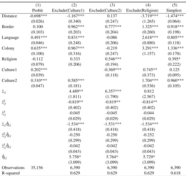
In addition to our main results, we confirm the validity of our excluded variable

. Table 2.9 reports the results for a robustness check. Column (1) reports the estimation result of selection equation. Columns (2) to (4) report the estimation result of outcome equation using Culture1, Culture2, and Religion as excluded variables respectively. Column (5) reports the estimation result of uncorrected selection and endogeneity biases (excludes all zero samples). We regard the estimation result in column (2) as our benchmark.

In column (3), we use Culture2 as an excluded variable instead of Culture1. Observing the regression coefficient signs in column (3), we can verify that the estimation result is seri- ously misspecified. The coefficient signs of variable Distance, Language, and Colony are sign- reversed and become nonsignificant, and Culture1 has a negative effect on trade volume. This result is not intuitive. If this is correct, the distance between two countries does not act as a proxy of transportation costs. The linguistic differences and colonial ties do not affect the consumers’

choice. This unexpected result does not support the hypothesis that Culture2 is the appropri- ate excluded variable. Moreover, we cannot explain why Culture2 does not affect the volume of music traded using our assumption of devotees and masses. We conclude that Culture2 is inappropriate to be used as an excluded variable, compared to Culture1.

In column (4), we exclude the Religion as in the Helpman et al. (2008) study. Here, the coef-

18

We also check the robustness of estimation model. We do poisson pseudo maximum likelihood estimation and

obtain similar result.

ficient values are overestimated and the standard errors are larger than benchmark ones, although coefficient signs are appropriate. This result implies that using Religion as an excluded variable causes exaggerates estimated coefficients. For example, the result in column (4) represents that two countries that share the same language trade about 13 times (=exp(2.618)) more on average compared to the two countries that do not share the same language. However, the average trade volume in a group that does not share same language is 188,637 copies, and the volume in a group that shares same language is 256,745 copies. The same tendency can be found in other variables. From this fact, we conclude that Religion cannot be utilized to satisfy the exclusion restriction in the case of music trade.

Choosing an adequate excluded variable is difficult empirical works. Our justification to use Culture1 as an excluded variable is not strong. However, we show that it is inappropriate to exclude other variables. Compared to others, the estimation result when excluding Culture1 appears to be reasonable. This validates our choice of the variable to exclude.

2.6 Conclusion

The purpose of this study is to reveal the relationship between cultural differences and trade of music. Cultural differences are an important determinant of music trade. We empirically confirm its effect by using a large dataset of music trade from about 188 countries.

To define the cultural differences, we review studies on ethnomusicology and politics, and identify cultural variables that represent the differences of music and mass culture. We use the modified gravity model of trade proposed by Helpman et al. (2008) to avoid the possible bias.

We assume that music consumers can be classified as devotees and masses, and that the number

of masses is much larger than devotees. This unique assumption helps Culture1 to satisfy the

exclusion restriction in our model.

From our estimation result, we find that the cultural differences play an important role when countries trade music, ceteris paribus. The cultural difference of music acts as a fixed cost, which has a positive effect on the probability of trade occurrence, but does not have a significant effect on the volume traded. The cultural difference of masses acts as a variable cost. If two countries share the same culture, they trade significantly more compared to the country pairs that do not share the same culture.

In addition to our full sample analysis, we also analyze the trade of music using the Western- Latin and Asian subsamples. In the Western-Latin region, the music culture variable Culture1 does not have a significant effect on the probability of trade occurrence, and both the Culture1 and Culture2 have no significant effects on the volume of music traded. This result implies that in the Western-Latin region, people do not care about the cultural differences when they consume music. In the Asian region, both cultural variables have no significant effects on the probability of trade occurrence and the volume of music traded. In addition, the productivity term ˆ z

, ˆ¯ η

, and their cross terms have no significant effect on the music volume. We conjecture that people do not focus on the cultural proximity or productivity in the Asian region.

In conclusion, we show the importance of cultural differences. Our estimation results demon- strate that the cultural differences play an important role in music trade although they do not have a significant effect when we limit the subject of analysis to specific samples. Moreover, one cultural variable can be treated as excluded variable and this helps us to satisfy the exclusion restriction of our two-stage estimation procedure.

Our study sheds some light on the role of cultural differences in the trade of cultural goods;

however, three issues remain open for future research.

Firstly, the results of this study cannot be directly applied to other cultural goods, such as

movies or books, mainly because we define one cultural variable in the context of music. Nev-

ertheless, our findings contribute to the literature by revealing the relationship between cultural differences and the trade of cultural goods. Further research on the relationship between cultural differences and other cultural goods is needed.

Secondly, we need to consider the effect of digital music trade and streaming service. Be- cause of the difficulty to trace the complete digital music flows, we choose a sample period when digital music trade and streaming service do not have significant impact on our estimation results and conclusion. However, the share of digital market is equivalent to physical one in 2014 and has tended to increase through the year. Some studies treat the digital music sales and trade, for example, Gomez-Herrera et al. (2014) use digital music sales data in US, Canada and 16 Euro- pean countries from 2006 to 2011 and investigates what drives digital trade patterns. Aguiar and Waldfogel (2015) obtain the volume of streams data from “Sportify” over the period of 2013–

2015 and examine the impact on the physical goods sales and the digital piracy. Although in many countries the data of digital music and streaming service flow are not completely avail- able, analysis and studies based on these data are helpful to reveal the role of cultural differences in cultural goods trade. Developing a way for tracing the digital music flows and analyzing them are topics for further research.

Finally, the effect of IPR protection (including copyright protection) must be investigated.

Although Shin et al. (2016) show the relationship between trade value and IPR protection, the

relationship between cultural goods trade and IPR protection is still unclear. In this paper, we

control the effect of IPR protection using fixed effects. However, we cannot identify the effects

themselves in the fixed effect terms. Investigating the relationship is also an important further

research topic.

2.7 Appendix

In this section, we will explain how to treat the incidental parameter problem of our two-stage estimation procedure. Our estimation procedure contains two equations.

First, we estimate the trade decision equation. The problem is occurred because our model has fixed effects of importer and exporter. This is the typical case of incidental parameter prob- lem. Fern´andez-Val and Weidner (2016) propose the bias correction way for nonlinear models that contain two-way fixed effects and we follow their way to correct the bias. The criterion function of first stage equation is

Q

=

∑

∑

f

( θ

, α

, γ

;X

), (2.8) where θ

is a K × 1 parameter and α

, γ

are fixed effects country i and j respectively.

Fern´andez-Val and Weidner (2016) show that for the bias corrected estimator

θ ˜

= θ ˆ

− W

(B

+ B

), (2.9) it is guaranteed that

√ IJ( θ ˜

− θ

) − →

N(0, Σ

). (2.10) This is the strictly exogenous components of X

case. For the detail of correction terms W

, B

, and B

, see Fern´andez-Val and Weidner (2016).

Then, we estimate the outcome equation. The two-stage estimation bias correction way with one-way fixed effect is proposed in Fern´andez-Val and Vella (2011). We expand their way to our two-stage estimation with two-way fixed effects model. The criterion function of second stage equation is

Q

=

∑

∑

f

( θ

, ζ , α

, γ

;X

, λ

) (2.11) where θ

is a M × 1 parameter vector, λ

is a L × 1 control variables vector, and ζ is a L × 1 coefficient vector. In our case, λ

can be written as λ

= (z

, z

,z

,z

η

, z

η

,z

η

, η

). We can show that for the bias corrected estimator

θ ˜

= θ ˆ

−W

(B

+ B

), (2.12) it is guaranteed that

√ IJ( θ ˜

− θ

) − →

N(0, Σ

), (2.13) where

W

=

∑

∑

d

· ( X ˜

λ ˜

)

· ( X ˜

λ ˜

)

(2.14)