GEO Debris and Asteroids
Toshifumi YANAGISAWA*1, Hirohisa KUROSAKI*1 and Atsushi NAKAJIMA*1
㊀ߨวࠊߖᴺ㧦ᓸዊ㕒ᱛ࠺ࡉ߮ዊᖺᤊߩᬌᴺ*
ᩉᴛ ବผ*1, 㤥ፒ ਭ*1, ਛፉ ෘ*1
Abstract
We established a new method that we call “the stacking method” to detect faint objects on CCD images such as unknown small size of GEO debris and undiscovered asteroids which include earth-crossing ones. A middle size of telescope and a normal CCD camera are enough to realize a fine result of the method. Many CCD images are used to detect faint objects. With this method, background stars are completely disappeared and the sky background fluctuation decreases extremely. This means faint objects, which are not visible on a single image, are detectable.
We evaluated this method using actual observation images taken by a 35cm telescope of Mt.Nyukasa Astronomical Observatory and a 2K2K back-illuminated CCD camera. We created two algorithms for the evaluation. One is for detection of GEO debris and the other is for that of asteroid. Both algorithms worked well and proved the effectiveness of this method. This method will contribute significantly to the safety of active satellites from collision of space debris, to search for near-Earth objects and to solar-system astronomy.
1. Introduction
Since Sputnik, the world's first successful satellite, was launched in 1957, humans have launched many satellites;
thus the number of artificial objects in orbit has been increasing. Explosions and collisions of these objects create large volumes of space debris. For the safety of people and satellites, this debris needs to be detected and cataloged.
Systems for observing space debris have been established in the United States and Russia[1]. Some four million pieces of space debris larger than 1mm are believed to exist, but less than 10 thousand pieces of them have been cataloged[2].
In the geostationary orbit, a minimum size for detection of about 50cm is a serious problem. Breakups near the orbit were reported in 1978, 1992, and 1994[3], and this debris spreads out to every longitude of the geostationary orbit, increasing the danger of a second collision. Strengthening the systems for observing GEO debris smaller than 50cm is critical to prevent the occurrence of these types of phenomena.
On the other hand, many groups are trying to observe near-Earth objects (NEOs) with the potential to collide with the Earth[4][5]. Observations of small asteroids in the main-belt or far ones, like Edgeworth-Kuiper belt objects, also help us to investigate the origins of the solar system
[6][7].CCD cameras are the most important tool for these purposes. Recently, the size of CCD chips has expanded to 2k×4k pixels, and a number of such CCD chips can be installed in a single CCD camera[8]. Scientists must analyze enormous volumes of data to get an outcome. Automatic detection is a desirable way to analyze data rapidly and accurately. Our group started test observations of GEO debris and asteroid in 1999. A 35cm telescope and a 2K2K back-illuminated CCD camera were set up at Mt.Nyukasa Observatory in Nagano Prefecture, Japan in 2002. We are developing algorithms to detect unknown GEO debris and undiscovered asteroids by using the actual observed data [9].
In this paper, we describe a new technique that we have named the stacking method for detecting small pieces of GEO debris. A large number of CCD images are cut out to match a target movement and a median image is created from these sub-images. This process removes the effects of fixed stars and enables to detect very dark objects not visible on a single CCD image. We used this technique to analyze actual CCD images and confirmed its effectiveness. In the first half of this paper, we describe the algorithm that is developed for detection of small pieces of GEO debris, its test observation and the result. In the second half, we describe the case of undiscovered asteroids.
* Received 3 December, 2007
*1 Advanced Space Technology Research Group, Institute of Aerospace Technology
2. The stacking method for GEO debris 2.1 General idea
GEO debris moves among fixed stars in the sky. In this paper, GEO debris does not mean debris that is exactly on the geostationary orbit but is around it. This means the GEO debris moves in the sky because of its inclination, semi-major
axis and/or eccentricity. Usual observations of GEO debris require a short exposure frame (a few seconds) without an equatorial movement of a telescope. Point sources as GEO debris in the frame are searched. Fixed stars create streaks on the frame. A long exposure time is needed to detect dark GEO debris, but as the exposure time becomes longer, the streaks of fixed stars extend beyond the frame and new fixed stars enter it. These obscure the weak light from small GEO debris.
As a result, the exposure time is limited to a few seconds.
This process does not detect dark GEO debris below the one frame limiting magnitude.
Taking a median value of many frames with a short exposure solves the problem. The median is the central value of multiple values. For example, 3 is the median among 1, 2, 3, 4, and 100. If the number of values is even, the median value becomes the average of the two middle values. As described in the above example, taking a median eliminates any effects from an unexpectedly high signal (in this paper, streaks of stars). On the other hand, the average of 1, 2, 3, 4, and 100 is 22, i.e., it is affected by the high value, 100.
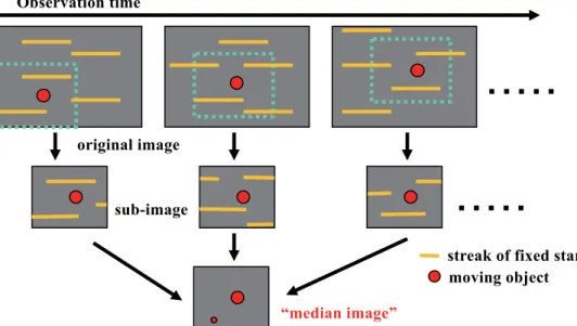
As shown in Figure 1, the stacking method cuts out sub-images from many CCD images to fit GEO debris movement. A median image of all the sub-images is then created. In this method, photons from objects are accumulated on the same pixels of sub-images and streaks of fixed stars are completely removed by taking the median because they are moving on the sub-images. Figure 2 shows an example of debris detected using the stacking method. Figure 2 (a) shows a part of one CCD image and Figure 2 (b) the same region of the final image after the process has been carried out. Fifteen Figure 1: Process of the stacking method
“median image”
䊶䊶䊶䊶䊶 䊶䊶䊶䊶䊶
Observation time
original image
sub-image
streak of fixed star moving object
(a)
(b)
Figure 2: An example of debris detected using the
images are used. It is difficult to confirm the presence of the debris in Figure 2 (a), whereas the debris is bright and no streak of fixed star exists in Figure 2 (b).
The background noise was reduced as in Equation (1).
(1)
Here N is the number of sub-images used to make up a median image. This means darker objects are detectable as more images are used. The factor 1.2 is calculated from Monte Carlo simulations [10].If the average is used instead of the median, the factor is 1.0. The average is slightly more powerful than the median in respect of the detection of unresolved asteroids. However, the median has the advantage of eliminating extremely high noises, such as cosmic rays and hot pixels that remain in an average image. Figure 3 shows the background noise levels for the number of median images.
The horizontal axis shows the number of stacked images, and the vertical axis the standard deviation of the sky background in analog-to-digital units (ADU). The dashed line represents Equation (1). The noise level is reduced as many images are used. Figure 2 and 3 show that the stacking method is able to detect very dark GEO debris that is invisible on a single CCD image. In order to detect invisible GEO debris on one image, various movements of the GEO debris are assumed and many processes as shown in Figure 1 are needed.
2.2 Test Observation
We tried a test observation of the stacking method in order to evaluate its effectiveness for detection of GEO debris.
Japan Aerospace Exploration Agency (JAXA) possesses an optical observatory site at Mt. Nyukasa, Nagano Prefecture, for research on GEO debris and asteroid observation technologies and data analysis processes [11]. The site is at 138q10̡30̢E, 35q54̡00̢N, 1810m altitude. There are a 35-cm telescope and a 2K2K CCD camera at the site.
The telescope is an H 350N manufactured by Takahashi Co.
Ltd. Its focal length is 1248mm. It is set on a fork-type equatorial mount 25 EF manufactured by SHOWA. The CCD camera is a FCC-104B, manufactured by Nakanishi Image Laboratory Inc., using a back-illuminated chip, the EEV’s 4240. Readout time of the CCD camera is about 10 seconds.
The total sky coverage of the image area of the system is around 1.27q1.27q, and its pixel scale is 2.2̢. The telescope and the camera are shown in Figure 4. The observation was carried out on February 6, 2003. We observed one region on the geostationary orbit without an equatorial movement of the telescope. The coordinates of the region was Az = 174.9, El = 48.3. 150 images were taken with a 10-second exposure time. The readout time of the CCD camera is about 10 seconds. 3 dark images were taken before the observation. We also took a 1-second exposure image in order to determine the accurate observed position. In this image, streaks of fixed stars are so short that we can identify
individual median
N V V 1.2
Figure 3: The background noise levels for the number of median images.
Figure 4: The telescope (35cm Newtonian telescope H 350N manufactured by Takahashi Co. Ltd.) and the camera (2K×2K back-illuminated CCD camera FCC-104B manufactured by N.I.L. Co. Ltd.) used for the observation.
them with normal star shapes and compare their pixel coordinates to the guide star catalog. The weather condition was very good and the observation was not bothered by any significant clouds. At twilight time, we got flat field images by taking the twilight sky images.
2.3 Analysis and Results
The data is stored in the local hard disk and later processed offline. The software IRAF (Image Reduction and Analysis Facility)[12] was used for the image processing concerning the stacking method. The IRAF can be carried out with the script mode. We developed an automatic analysis process of the stacking method using the IRAF, a script language perl and C language.
Figure 1 shows the simplified case of the stacking method for better understanding. Many processes should be carried out especially for the detection of dark objects below the background noise levels in practice. First, all the images were dark-image subtracted for reducing the electric noises and flat-fielded for adjusting the sensitivity differences between each pixel. The subtracted dark image is the median image of 3 dark images taken at the beginning of the observation. The cosmic-ray free dark image is constructed by taking median of 3 dark images.
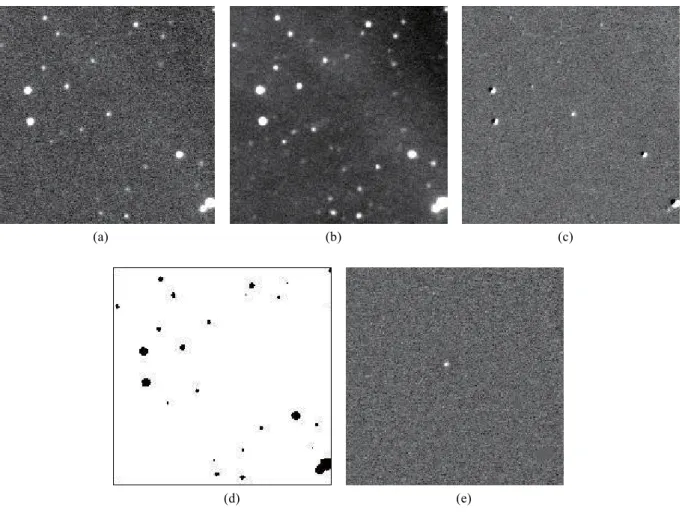
Second, the sky level of each image is adjusted. The atmospheric condition usually changes the brightness of the sky. In order to detect very dark objects around the sky background level, the sky level of each image must be adjusted accurately. Furthermore, our CCD camera reads out its data from two outputs for the fast readout. This makes some difference of the sky background level between the left and the right side of the image as show in Figure 5 (a). We investigate two parts of the sky level(the left and the right side) of all the images using the median values of 200×200 pixels of each region and adjusted the sky level. Figure 5 (b) shows one image whose sky level is adjusted. The sky level difference between the left and the right side region is eliminated.
Although we use median images in order to eliminate the streaks of fixed stars, the influences of the streaks of bright stars remain as shown in Figure 5 (c). We ignored high value regions using an appropriate threshold value. Figure 5 (d) shows one image after ignoring high values. The value of the shy level is applied at the ignored regions. Figure 5 (e) represents the median image made from the high-value ignored images. The influences of the streaks of bright stars are totally eliminated.
We apply dark frame subtractions and flat-fieldings toward all the images. However, in some cases, these processes do not work well. Figure 5 (f) is the median image of all the observed images. Intervention patterns that are usual for back-illuminated CCD chips are appeared and there are dark parts at the four corners. Those are caused by the insufficient flat-fielding. It is very difficult to construct a perfect flat-field frame. We subtracted the image of Figure 5 (f) from all the observed images in order to eliminate these effects.
After applying all the processes as mentioned above to all the observed images, the stacking method is carried out. In order to detect invisible GEO debris on one image, various movements of the GEO debris are assumed and many processes as shown in Figure 1 are needed. Various types of space debris are crossing the observing field. If we try to detect all of the debris, a vast number of processes are needed and that is not realistic for the present machine calculating ability. We concentrate to detect GEO debris that has a proper inclination. The movements of such debris are almost vertical.
We only searched objects moving almost vertical directions in the field. When the GEO debris has a high inclination, it moves fast and a short number of images are required to detect it. We divided all of the 150 images by a few sets in response to various speeds of GEO debris. We prepared 6 sets of 25 images, 3 sets of 50 images and 2 sets of 75 images. In order to confirm that the candidate is real GEO debris, we set a criterion that two detections in two serial sets are needed.
We changed the shift values of targets by 3 pixels to detect dark GEO debris. The shift values means the movement of the GEO debris from the first image of the set to the last one.
We carried out about 8000 processes for one set. The detection threshold of the GEO debris is 4 times of the background noise of the median image of the set. If one candidate is detected, the real shift value is searched around the detected shift value until the peak value of the candidate is the maximum. This process does not take time because small images around the candidate are used. We used two PC workstations DELL Prescision 340 for the analysis. This machine has one Pentium 4 CPU and 4 GB memories. OS is Red Hat linux ver.8. The time for analyzing one set for one PC is about 16 hours. It takes about 4 days to analyze all the sets of images. After all the candidates are picked up in all the sets, the pairs whose movements are coincident are searched.
We detected 10 candidates. Table 1 shows the details of the candidates. We can get the 4 positions of the candidates and the times when the candidates are at the positions. 4 positions mean the positions at the first and the last image of the first
set and those of the second set.
We also took a 1-second exposure image in order to determine the accurate candidate positions. In this image, streaks of fixed stars are so short that we can identify them with normal star shapes and compare their pixel coordinates to the guide star catalog. The IRAF ‘daofind’ command is
able to find out point-like shapes in the image and their pixel coordinates. From the rough values of observed Az, El and observed time of the image, we can calculate the rough celestial coordinates of the central position of the image.
Therefore, we can pick up the celestial coordinates of stars around the observed region from the guide star catalog.
(a)
(c) (d)
(f) (e)
(b)
Figure 5: Images produced during the processes of the stacking method.
No. Time(UT) X Y Az El Brightness(ADU) magnitude size(cm)
1 18:43:50 679 34 174.760 47.709 276.98 15.7 363 18:52:14 768 499 174.509 48.275 276.98 15.7 363 18:52:36 770 513 174.503 48.292 287.96 15.7 363 19:01:02 858 969 174.250 48.847 287.96 15.7 363 2 18:19:39 95 1020 174.300 47.640 9.33 19.4 66 18:28:04 93 723 174.239 48.009 9.33 19.4 66 18:28:25 88 723 174.230 48.009 9.18 19.4 66 18:36:50 106 441 174.209 48.361 9.18 19.4 66 3 18:28:25 902 27 175.632 48.969 9.63 19.4 66 18:36:50 914 309 175.701 48.619 9.63 19.4 66 18:37:11 918 293 175.707 48.634 10.64 19.3 69 18:45:36 924 561 175.759 48.307 10.64 19.3 69 4 18:28:25 809 41 175.458 48.942 9.21 19.4 66 18:36:50 809 311 175.503 48.606 9.21 19.4 66 18:37:11 796 316 175.479 48.598 10.02 19.3 69 18:45:36 798 593 175.529 48.254 10.02 19.3 69 5 18:28:25 746 58 175.342 48.914 9.16 19.4 66 18:36:50 752 328 175.400 48.579 9.16 19.4 66 18:37:11 748 326 175.391 48.580 10.96 19.2 72 18:45:36 769 598 175.476 48.245 10.96 19.2 72 6 18:45:57 105 400 174.198 48.411 10.13 19.3 69 18:54:21 114 688 174.272 48.055 10.13 19.3 69 18:54:37 105 695 174.257 48.045 10.67 19.3 69 19:03:08 121 1003 174.346 47.665 10.67 19.3 69 7 18:45:57 737 345 175.373 48.555 9.07 19.5 63 18:54:21 755 684 175.464 48.136 9.07 19.5 63 18:54:37 753 698 175.463 48.119 11.05 19.2 72 19:03:08 754 1022 175.518 47.716 11.05 19.2 72 8 18:37:11 903 338 175.684 48.583 7.00 19.7 57 18:54:21 930 683 175.789 48.156 7.00 19.7 57 18:54:42 937 671 175.801 48.172 7.69 19.6 60 19:11:53 948 998 175.873 47.767 7.69 19.6 60 9 18:19:39 81 414 174.157 48.391 6.46 19.8 55 18:45:36 111 402 174.211 48.410 6.46 19.8 55 18:45:57 109 396 174.205 48.417 6.39 19.8 55 19:11:53 118 372 174.218 48.448 6.39 19.8 55 10 18:19:39 502 878 175.026 47.867 9.06 19.4 66 18:28:04 481 452 174.912 48.394 9.06 19.4 66 18:28:25 484 443 174.916 48.405 9.27 19.4 66 18:36:50 484 29 174.842 48.919 9.27 19.4 66
Table 1: The details of the detected candidates.
The IRAF command ‘ccxymatch’ matches the pixel coordinates and the celestial coordinates of corresponding stars using the triangles algorithm and calculate the focal plane distortion cause by the optics of the telescope. The IRAF command ‘cctran’ is able to translate the pixel coordinates of the candidates to the celestial coordinates using the plate solution that ‘ccxymatch’ calculated. We then calculate Az and El values of them from the celestial coordinates. At that time we consider the precession and the nutation effects of the celestial coordinate system. We also consider the atmospheric effect that increases El values. We will be able to determine the orbit of detected GEO debris using these values.
The V band magnitudes of detected candidates are estimated using the V band magnitudes of background stars. The sizes of them are also calculated using the albedo value 0.1. We are able to detect about 50cm GEO debris by means of observations using the 35cm telescope and the CCD camera with the stacking method.
2.4 Discussion
As we showed in previous sections, the stacking method is powerful tool to detect very small GEO debris that is invisible on a single CCD image. If a larger telescope is used for the observation, smaller debris is detectable. A 1m telescope is able to detect about 30cm GEO debris (21 magnitude) using the stacking method. The Japan Space Forum has established the observatory, Bisei Spaceguard Center (BSGC) that is used solely for the observation of space debris and NEOs (near earth objects: asteroids and comets)[13][14]. It comprises one 1m telescope and one 0.5m telescope. Wide-field CCD cameras consisting of back-illuminated chips are installed on both the telescopes.
We would like to apply the method to the observation system of the BSGC in the future.
Although the stacking method is able to detect very dark GEO debris, it takes much time to analyze. For the practical use of the method, we need to reduce the analyzing time. The progress in the processing performance may help to reduce the time required.
We need to manage a number of detected GEO debris in the future. The accurate orbital determinations of all the GEO debris are required for that. We should detect GEO debris twice with an interval of a few hours or one day in order to determine the orbit of it. Furthermore, we have to observe many regions of the sky for many detections of unknown GEO debris. We need to consider the advantage and the
disadvantage of the stacking method, required accuracy for the orbital determination, characteristics of the observation system (for example, readout time, field of view of the CCD camera and pointing accuracy of the telescope.) and so on.
Then the best solution of the observation (number of field, images, exposure time, intervals and so on) must be found out for the practical. Umehara et al. found out a very efficient procedure that takes following things into considerations[15].
(A) A broad observation is realized by scanning GEO. (B) In order to carry out a systematic observation, surveyed range should be sorted according to orbital elements. (C) An efficient observation is considered to reduce operational costs.
This type of observation strategy must be established for the systematic observation and the management of GEO debris in the future.
3. The stacking method for asteroid
(a)
(b)
Figure 6: An asteroid detected using the method.
3.1 General idea
Asteroids and comets move against the field of stars in the sky. For example, main-belt asteroids move approximately 15' in one day and Edgeworth--Kuiper belt objects approximately 50''. The usual observation of an asteroid
Figure 7: Procedure of the method
requires a few frames in the same region of the celestial sphere at a proper time interval with the equatorial movement of the telescope. These frames are then compared to find moving objects against the star field. The exposure time is limited to about 5 mins because of asteroid movement. A visual inspection using a brink comparator or some programs of moving target indicator algorithm are used for the analysis.
These processes do not detect objects darker than the limiting magnitude of one frame. On the other hand, more sophisticated matched filter algorithms that can achieve better than the limiting magnitude are being developed by various groups[16][17].
The basic process of the method is the same as that for GEO debris described in section 2.1. Multiple CCD images are used to detect faint asteroids below the limiting magnitude of a single CCD image. Figure 6 shows an example of an asteroid detected using the method. Figure 6 (a) shows a part of one CCD image and figure 6 (b) the same region of the final image after the process was carried out. Forty images were used. It is impossible to confirm the presence of the asteroid in figure 6(a), whereas the asteroid is bright and no field star can be seen in figure 6(b). The differences of feature of background stars are seen between figure2 (a) and 6 (a).
This is because of the difference of the observation mode of the telescope. Relative motions of asteroids to background
stars are very slow. In such a case, observations are carried out in star-tracking mode. On the other hand, the relative motion of GEO debris is fast which requires the telescope to operate in stop mode. The method is not a simple shift-and-co-add one. It is impossible for the simple method to eliminate the effects of field stars, as shown in figure 6.
Several processes are included in the method, as explained below. All of the processes are constructed with Perl scripts and IRAF.
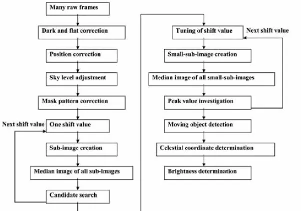
3.2 Detail of the method 3.2.1 The First Process
Figure 7 shows the entire procedure of the algorithm. Before the main process, an initial pre-processing is carried out to make clean input images for the main process. Multiple images of one sky region are taken with the observation equipment. First, all of the images are dark-frame subtracted and flat-fielded.
We then correct the mechanically induced position differences of each frame, using the pixel coordinates of one field star near the central region of the observed field. In practice, we set the first pixel coordinates and a search radius.
The algorithm searches for the brightest pixel within the circle. In the next image, the initial coordinates are changed to the coordinates of the brightest pixel found in the previous
image. These processes are continued through to the last image. Using coordinates based on the brightest pixel of each image, the algorithm crops the common regions from all of the images. In this correction, we use only one star, which means that rotation of the observed field during the observation is not corrected in order to simplify the method.
The sky levels of each image may differ because of variations in the atmospheric conditions. The algorithm corrects any differences. We specify one small region (e.g., 5050 pixels) around the center where there is no field star.
The algorithm investigates the median values and the standard deviations of this region in all of the images. The average of the median values is calculated, and constant values are added to or subtracted from all of the images so as to adjust the sky level of this region to the average value. The
sky level differences of each image are almost completely corrected by this process.
As mentioned in subsection 3.1, the method is not a simple shift-and-co-add method. Even if a median image of all the sub-images is created, the influences of field stars must remain, because the motion of the target relative to field stars is small. Therefore, the algorithm removes field stars in advance. This process is somewhat complicated. First of all, the median image of all the images is created. This is not a median filter that is normally used in image processing. A median filter is applied to one frame to eliminate noises (especially spiky ones) by taking median values of some local pixels. In our algorithm, one pixel value of a median image is a median value of all raw images' same position values.
Therefore, one median image is created from all raw images.
(a)
(d) (e) (c)
(b)
Figure 8: Mask pattern correction. (a) Part of one raw image, with one asteroid visible in the center. (b) Same part of a median image of all raw images; the asteroid has disappeared. (c) Equals (a) minus (b). Most parts of most field stars are removed. Central parts of bright stars remain because of PSF difference in each of the images and sub-pixel position mismatching of the images. (d) A mask-pattern created from (b) applying the proper threshold value. (e) Result of the mask pattern application. The influences of field stars are completely removed and only the asteroid remains.
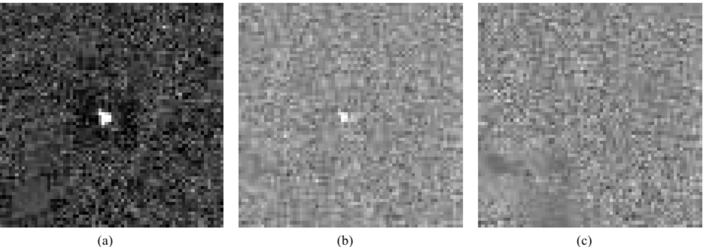
Figures 8(a) and 8(b) show a part of one raw image and the median image, respectively. In the median image, the signal-to-noise ratio is improved as described in equation (1), making some faint stars not visible on the raw image visible.
Moving objects disappear in the median image because their positions are different in each image. There is one asteroid at the center of figure 8(a) that is completely removed in figure 8(b). Therefore, taking a median of all the images makes moving-object-free and very low-noise image. By subtracting the median image from all the images, it is possible to remove field stars. If there are some sky-level inclinations caused by the poor flat-fielding and/or Moon, those are also removed by this process. However, influences from the central regions of bright stars remain because of PSF (point spread function) differences in each of the images and position mismatching between each of the images of less than one pixel. Figure 8(c) shows figure 8(a) minus figure 8(b). The asteroid remains in figure 8(c), but influences from the central regions of bright stars also remain. In order to remove such influences, the algorithm prepares a mask pattern that ignores the influenced
regions. The mask pattern is made from the median image by applying a threshold value. The threshold value is determined as a few times (e.g., four times) of the standard deviation derived at the sky level adjustment. Figure 8(d) shows the mask pattern where higher regions than the threshold value are colored black and the others are white. The mask pattern is applied to all of the images. In practice, no values (zero) are set in black regions, and nothing is done to white regions.
Figure 8(e) shows the result of mask pattern application. The influences of field stars are completely removed, and only the asteroid remains. In other words, this mask pattern process ignores the bright regions in images. This is quite reasonable, because if asteroids are near those of bright stars, it is difficult to confirm them. This also removes image contamination caused by trails of field stars. In the simple shift-and-co-add method, unusable region caused by trails of field stars increases as the observation time increases. In this algorithm there is no such effect. By subtracting the median image, moderately bright regions are clearly removed, and such regions are usable for the detection of moving objects.
3.2.2 The Main Process
In the first process, the algorithm prepares very clean and field-star-free images. We then specify shift values for the x- and y-axes of images in pixels. Once the shift values are determined, the algorithm crops sub-images from all of the images to fit the values, as shown in figure 1. The area of the sub-images depends on the shift values. If the shift values are 100 and 50 pixels for the x- and y-axes, respectively, the area of the sub-images is (Nx-100)(Ny-50) (Nx and Ny being the
number of pixels of the raw images along the x- and y-axes, respectively). A median image of all the sub-images is created and the candidates for moving objects are searched. At this stage, some readers may think that we should use average (or sum) instead of median, because we eliminate field stars clearly in the first process. However, some spiky noises, such as cosmic rays, hot pixels, blooming, and variable stars, must remain in individual frames that affect the average (or sum)
(b) (c) (a)
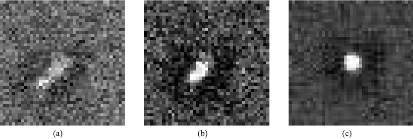
Figure 9: Difference between an average (or sum) image and a median image. (a) Part of one raw image, with a cosmic-ray effect in the center. (b) Same part of an average image of all raw images.
The cosmic ray effect remains significantly. (c) Same part of a median image of all raw images. The effect is completely removed.
image seriously. A median image is not affected by such noises. Figure 9 shows the difference between an average (or sum) image and a median image. The effect of a cosmic ray of one raw image figure 9(a) remains on the average image figure 9(b), not on the median image figure 9(c). We know that the median reduced the noise levels as equation (1).
Therefore, we chose median to avoid false detection. In order to find candidates, two criteria are assigned. One is a threshold value that is a few multiples of the background noise of the median image calculated by equation (1). We can specify the threshold value according to the situation. If the search goal is quite faint moving objects, the threshold must be low, which may detect false candidates and be time-consuming to analyze. The other criterion is the shape parameter, defined as the ratio of the value of the brightest pixel to the total value of the nine pixels centered by the brightest one. If the shape parameter is smaller than the specified value, the candidate is regarded as being noise. The shape parameter approaches unity as the PSF becomes small.
We can also specify this value according to the observation system and the atmospheric conditions that affect the PSF.
Many shift values must be applied to disclose various moving objects. If there are candidates that satisfy the two criteria, the algorithm records its coordinates on the first image and the shift values as a candidate. We call this the first detection
Once a candidate is detected, the algorithm searches for the true shift values. Small regions (e.g., 2020 pixels) around the candidate are cropped from all of the images, with a small change in the shift value. A median image of all those small sub-images is created and the peak value of the candidate is
investigated. This is repeated at shift values within r3 pixels along the x- and y-axes from the detected shift value.
The shift value that shows the highest peak value becomes the next shift value. The same process is carried out for the next shift value. These processes are repeated until the peak value becomes a maximum at the true shift value. The shape parameter is calculated simultaneously. The algorithm records the coordinates of the first image, its true shift value, and the shape parameter as a detected moving object. At this time the shape parameter naturally meets the criterion. We call this the second detection.
In order to detect faint moving objects, the algorithm needs to explore various shift values with small steps because such objects will disappear with a small change in the shift value.
However, we cannot analyze all shift values because the analysis time is limited by the machine power. We therefore have to thin out shift values for analysis. We discuss this effect in section 3.4.
Bright moving objects are detected with various shift values in the first detection process, with an elongated shape as shown in figure 10(a). In the second detection process, they approach the true shift value, as shown in figures 10(b) and 10(c). Many second-detection processes are repeated for one bright moving object, which is a time burden for the analysis.
We therefore set a territory for the second-detected object to avoid this. During the second-detection process, the algorithm refers to the coordinates of the second-detected objects. When the coordinates of a currently analyzed object are inside the territory (e.g., 20 pixels) of a second-detected object and its brightness is less than that second-detected object, the algorithm stops the analysis, judging that the object has
(a) (b) (c)
Figure 10: Bright moving objects are usually detected at different shift values in the first detection, showing an elongated shape, as (a). Then, they gradually approach a true shift value, as (b) and (c).
already been second-detected. If the brightness of the analyzed object is brighter than the second-detected object, the algorithm deletes the second-detected object as a false candidate and continues the analysis until the brightness of the analyzed object reaches a maximum. This also avoids missing of a brighter moving object near a false object caused by a low threshold level setting. This criterion cannot detect two near-neighbor moving objects (only the brighter one is detected), but such a situation is very rare. The size of a territory is determined by the machine power, the limiting magnitude, the pixel scale of the observation system, and so on forth.
Finally, the method determines the celestial coordinates of the detected object using the Guide Star Catalog[18]. Pixel coordinates of field stars in the median image created in the first process are investigated using the IRAF command
“daofind”. These coordinates are compared with those in the Guide Star Catalog, and the plate solution is calculated using the IRAF command “ccxymatch”. We can specify the pixel coordinates of detected objects at the beginning and the end of an observation using the coordinates and the shift value recorded at the second detection. Converting these coordinates to the celestial ones, using the plate solution and the IRAF command “ccxytran”, is the simplest. However, the celestial coordinates determined include a one-pixel size error that may correspond to a few arcsec for wide field optics.
Such an error limits the precision of orbital determination.
The algorithm therefore calculates the two central coordinates at certain intervals (e.g., 20 minutes) by linearly scaling the coordinates of the beginning and the end. This will reduce any positional errors to less than 1Ǝ. The magnitudes of detected objects are also determined by comparing the magnitudes of field stars in the median image with those given in the Guide Star Catalog. After checking whether the detected objects are known or unknown using MPChecker[19], we can report the observation time, the celestial coordinates, and the magnitude of detected objects to International Astronomical Union (IAU).
3.3 Test Observation
We performed a test observation to evaluate the effectiveness of the method for detections of asteroids. The same observational equipments for the observation of GEO debris are used. The detail of the observation equipments are described in section 2.2.
We observed three main-belt regions on 2002 March 12 and
13; 40 images with 3-min exposure were taken for each of the regions. The atmospheric conditions were fairly good. The PSF of the field star was 5.2̢. The limiting magnitude of one frame was 19.5 magnitude with SN 10.
We analyzed these data with the algorithm at various shift values. Asteroids whose daily motions are 5.95ƍ-31.75ƍ with any directions of motion, except retrograde, were detectable.
These shift values were set to a 5-pixel step in order to save analyzing time. Four hundred shift values were applied, requiring 2 hr to analyze one field (40 frames of 2K×2K pixels images) with a “Precision 340” PC manufactured by DELL. This PC contains 3.06 GHz CPU and 2 Gbytes memories. The total analysis time was 12 hr. The threshold value for the mask pattern was 28.0 analog-to-digital unit (ADU). This value is not needed to determine so strictly. As can be seen in figure 8 (c), only the central regions of the bright stars remain. Therefore, 2-5 times the sky background fluctuation in one frame is sufficient. At more crowded regions with the field stars, the threshold needs to be high to obtain no-masked regions. We set the detection threshold at 18.0 ADU, or 1.3-times the sky background fluctuation in one frame, and the shape parameter to 3.0. The detection threshold should be determined carefully. If the search goal is quite faint moving objects, the threshold must be low, which may detect false candidates and be a time-consuming analysis.
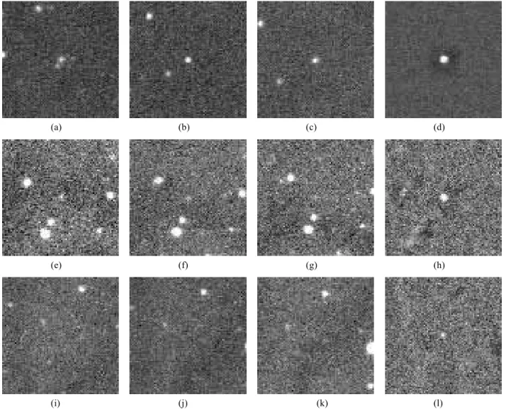
From our experience, 5--6 times the sky background fluctuation in the median frame of all raw images produces good results. We discuss this point in section 4. After detecting candidates from all of the fields on both days, pairs whose starting and stopping positions were aligned within 1 arcsec along the observation time were discovered to be real asteroids. The candidates that have no partners may be false detections or real asteroids that were not detected on both days for some reason. Table 2 gives the details of 16 asteroids detected with the algorithm. The magnitudes were estimated from those of field stars that are listed in the Guide Star Catalog. Some examples are shown in figure 11. NAL019 are almost invisible on the raw images. We reported these 16 asteroids to IAU. NAL015, NAL016, NAL017, NAL018, and NAL019 are newly discovered asteroids. They are registered as 2002EQ153, 2002ES153, 2002EU153, 2002ER153, and 2002ET153. We demonstrated that a 35-cm telescope was able to detect a 21 magnitude asteroid with the method.
(a) (b) (c) (d)
(g)
(e) (f) (h)
(k) (l) (j)
(i)
Figure 11: Three asteroids detected in a test observation. (a)-(c) and (d) are raw images of asteroid 18564 (18.7 mag) and the final image of the algorithm, respectively. The asteroid is at the center of each image. Images (e)-(g) and (h) are those of asteroid 40491 (20.5 mag). Images (i)-(k) and (l) are those of NAL019 (21.7 mag). 18564 is clearly visible in the raw images. In contrast, 40491 is hard to see and NAL019 is invisible in the raw images. Images (h) and (l) show that the algorithm successfully disclosed these faint objects.
3.4 Detection Efficiency
With a test observation, we demonstrated that the method is able to detect faint moving objects that are invisible on a single frame. For serious science work, we should know the detection efficiency of the algorithm. For example, the efficiency is needed to estimate the size and spatial distribution of main-belt asteroids or Edgeworth-Kuiper belt objects [20]. We used raw frames taken in the test observation to calculate the detection efficiency. First, these frames were randomly re-arranged with respect to their observation time, in order to eliminate the possibility of real asteroid detection events. Then, artificial asteroids of various magnitudes were placed on these frames with the proper shift values. Figure 12 shows artificial asteroids of various magnitudes. By analyzing these frames with the algorithm, we investigated
the detection efficiency under various conditions.
Figure 13 shows the detection efficiency with various numbers of frames processed by the algorithm. The x- and y-axes are the magnitudes of artificial asteroids and the detection efficiency, respectively. The figure indicates that fainter objects are detectable as the number of frames increases. The detection threshold of figure 13 was determined to be 6-times the background noise of the corresponding number of images as shown in figure 3.
We then investigated the influence of the detection threshold value. Figure 14 shows the detection efficiency at various threshold values; 40 frames were used in the method. Darker objects are detectable as the threshold value decreases.
However, figure 15 indicates that false detections increase as the threshold value decreases. The values in figure 15 are for
Figure 13: Detection efficiency with various numbers of frames processed by the method.
Figure 15: Number of false detections at various threshold values.
(a) (b) (c)
(d) (f) (e)
(h) (i) (g)
Figure 12: Artificial asteroids used to calculate the detection efficiency. Images (a), (b), and (c) show a 19.5 mag asteroid.
The asteroid is in the center of the circle of (a). Images (d), (e), and (f) show a 20.5 mag asteroid. Asteroids are in the same position as in (a), (b), and (c). Images (g), (h), and (i) show a 21.2 mag asteroid.
Figure 14: Detection efficiency at various threshold values. Figure 16: Detection efficiency for various step size of the
one shift value. When 400 shift values are investigated, as in this test observation, the values in figure 15 are multiplied by 400. A low threshold value should be used to detect faint moving objects, but this causes many false detections, which require extended analysis time. Powerful machines are needed to cope with this.
As described in subsection 3.2.2, the method needs to survey various shift values with a small step to detect faint moving objects, because such objects will disappear with a small change of the shift value. However, we cannot analyze all shift values because of the excessive computational demand. We investigated the detection efficiency for various step sizes of the shift values. Forty frames were used in the algorithm with a threshold value of 16 ADU. Figure 16 shows the results. NN means the shift values are changed by N-pixel steps. Fainter moving objects are difficult to detect as the step size increases. However, the number of process decreases by NN as compared with the 11 case. This reduces the analysis time by a factor of NN, as compared with the 11 case. The user of this method can specify the most suitable parameter settings (frame number, threshold, and step size) for the observational goal, equipment capability, field number, observation frequency, and machine power.
As described in section 3.3, the limiting magnitude of one frame of our observation system is 19.5. Figure 13 shows that the algorithm can detect 2-mag fainter objects using 40 frames. However, the method requires many frames, which means that the area coverage in a night is reduced. Various NEOs search groups observe one field 3 times, and survey a wide field in a short period to detectas many NEOs as possible. After they find out all NEOs that they can detect in present observation mode, we think our method is useful to obtain a 2-mag deeper limiting magnitude which means smaller NEOs are detectable. In this case, a 13 (40/3) times observation period is needed to cover same field of present observation mode. However, this disadvantage is recovered by multiplying the same observation equipment or extending the waiting time for the result, which are negligible compared with a catastrophe caused by an Earth impactor.
We have transferred our techniques for the algorithm to a company, AstroArts Inc., and collaborate with the company to produce a user-friendly program for discoveries of asteroids,
``Stella Hunter Professional'', which embodies the method described here [21]. This is written in C++ and GUI based. It runs on Windows 98SE, Me, 2000 and Xp machines. At least, 1 GByte hard disk and 256 MByte memories are need for machines. During development process of this program, a lot of asteroids were discovered by this method. The details of the discovered asteroids are listed in the appendix.
4.Conclusions
We established the stacking method in order to detect unknown small size of GEO debris and asteroids. This method uses many CCD images and enables us to detect very faint objects that are below the detection limit of one CCD image. Sub-images from many CCD images are cut out in order to fit the movement of the objects. A median image of all the sub-images is then created. This eliminates the background stars and reduces the sky background noise efficiently. We tried this method using a 35cm telescope and a 2K2K CCD camera. In the case of detection of GEO debris, the method detected 20 magnitude objects that are about 50cm in the geostationary orbit with the albedo of 0.1. In the case of asteroid, 21 mag asteroids are detected by analyzing 40 images with this method. These results show this method works efficiently to detect faint objects.
Concerning analysis time, although it does not take much time to detect faint main-belt asteroids because their motions are almost same, it does for detection of faint GEO debris and NEOs. We need to find out an efficient strategy using the method for the future systematic observation of GEO debris and NEO surveys.
Table2: Details of detected asteroid
References
[1] National Research Council, Orbital Debris - A Technical Assessment, Commission Engineering and Technical Systems, National Academy Press, Washington, D.C., 1995.
[2] The Report on the Investigation about Optical Telescope for the Observation of Space Debris and NEO, Fundation for Promotion of Japanese Aerospace Technology(JAST) Press, 1997.
[3] Portree, D. S. F. and Loftus, J. P.: Orbital Debris: A Chronogy, NASA/TP-1999-208856, 142-146, 1999.
[4] Bottke, W. F., Jedicke, R., Morbidelli, A., Petit, J.-M., and Gladman, B.: Understanding the Distribution of Near-Earth Asteroids, Science, 288(2000), pp.
2190-2194.
[5] Talent, D. L., Maeda, R., Walton, S. R., Sydney, P. F., Hsu, Y., Cameron, B. A., Kervin, P. W., Helin, Eleanor F.; Pravdo, S. H., Lawrence, K., Rabinowitz, D.: New home for NEAT on the 1.2m/B37 at AMOS, Proc. SPIE, 4091(2000), pp. 225-236.
[6] Marzari, F., Farinella, P., and Davis, D. R.,: Origin, Aging, and Death of Asteroid Families, Icarus, 142(1999), pp. 63-77.
[7] Jewitt, D., and Luu, J.: Discovery of the candidate Kuiper belt object 1992 QB1, Nature, 362(1993), pp.
730-732.
[8] Miyazaki, S., Sekiguchi, M., Imi, K., Okada, N., Nakata, F., and Komiyama, Y.: Characterization and mosaicking of CCDs and the applications to the SUBARU wide-field camera (Suprime-Cam), Proc. SPIE., 3355(1998), pp. 363-374
[9] Yanagisawa, T., Nakajima, A., Kimura, T., Isobe, T., Futami, H. and Suzuki, M.: Detection of Small GEO Debris by use of the stacking method, Trans, Jpn Soc, Aero. Space Sci, 44 (2002), pp. 190-199.
[10] Pennycook, G.: Modification of the Boller and Chivens Telescope to f/6.25 and Photometry of IC5249's Halo, MS thesis, Univ. Auckland, 1998; Report of the work done with the Grant-in-Aid for International Scientific Research in 1996-1998, given by the Ministry of Education, Science, Sports and Culture of Japan, pp.
204-310, 2000.
[11] Nakajima, A., Kimura, T., Yanagisawa, T., and Hoshino, T.; GEO/LEO Space Debris Optical Observation Facilities in NAL, Proceedings of the 23rd International Symposium on Space Technology and Science, 2(2002), pp. 2336-2341.
[12] http://www.iraf.noao.edu/
[13] Isobe, S. and Japanese Spaceguard Association.:
Japanese 0.5m and 1.0m Telescope to Detect Space Debris and Near-Earth Asteroids, Advances in Space Res., 23(1999), pp. 33-36.
[14] Isobe, S., Mulherin, J., Way, S., Downey, E., Nishimura, K., Doi, I. and Saotome, M.: A Cost Effective, Advanced-Technology Telescope System for Detecting Near Earth Objects and Space Debris, Proc. SPIE, In Telescope Structures, Enclosures, Assembly / Integration / Validation, and Commissioning, 4004(2000), pp. 382-388.
[15] Umehara, H. and Kimura, K.: An optical search for near-synchronous debris: survey to 90 degrees of right ascension, J. Jpn. Soc. Aeronaut. Space Sci, 49(2000), pp. 1-8.
[16] Mohanty, N. C., IEEE Trans. on Pattern Analysis and Machine Intelligence, 3(1981), pp. 606
[17] Kelly, E. J., IEEE Trans. on Aerospace and Electronic Systems, 22(1985), 115
[18] http://www-gsss.stsci.edu/gsc/GSChome.htm [19] http://scully.harvard.edu/~cgi/CheckMP
[20] Yoshida, F., Nakamura, T., Watanabe, J., Kinoshita, D., Yamamoto, N., and Fuse, T.: Size and Spatial Distributions of Sub-km Main-Belt Asteroids, PASJ, 55(2003), pp. 701-715
[21] http://www.astroarts.com/products/stlhtp/index-j.shtml
Appendix