Transient Stability Regions of Power Systems: University of the Ryukyus Repository

(1)

Title

Transient Stability Regions of Power Systems

Author(s)

Miyagi, Hayao; Taniguchi, Tsuneo

Citation

琉球大学理工学部紀要. 工学篇 = Bulletin of Science &

Engineering Division, University of the Ryukyus.

Engineering(15): 105-114

Issue Date

1978-03-01

URL

http://hdl.handle.net/20.500.12000/27655

(2)

Transient Stability Regions of Power Systems

Hayao MIY AGI* and Tsuneo TANIGUCHI**

Summary

The direct method of Lyapunov is used to estimate the stability region

of power systems. A method for the construction of the Lyapunov function,

which has been developed recently, is applied to a

single-machine system with

and

without

a velocity governor. Such method is based

on

a construction

technique of the Lagrange's state function resulting from

second-order

ordinary

differential equations. The stability region given by the obtained Lyapunov

function is compared

with

those

given

by other Lyapunov functions and is

found to be useful in the power

system

transient stability problem

.

Furthermore,

its construction procedure seems to be concise.

List of principal symbols

M machine(generator) inertia constant in p.u. power second per electrical radian.

D = machine damping coeff;cient in p.u. power-second per electrical radian. Eq' = p.u. voltage proportional to field flux linkage.

EB = p.u. infinite-bus voltage.

xd p.u. direct axis synchronous reactance. Xq p.u. quadrature axis synchronous reactance. xd' = p.u. direct axis transient reactance.

X12 = p.u. total reactance between the generator terminal and the infinite-bus. Kg= loop gain of the governing system.

wo = 2 "fo Cfo=60Hz)

Tg = equivalent time constant of the governor, second.

1 . Introduction

1)

In the previous paper, the authors presented a new method of constructing Lyapunov functions for power systems represented by n second-order ordinary differential equations. The Lyapunov function constructed by the method :s equivalent to the generalized energy function of the system.

In this paper, the stability region given by the obtained Lyapunov function is compared with those g:ven by other Lyapunov functions. To begin with, a simple model of power system without,:velocity governor is considered. Then, the various Lyapunov functions are derived for the system. Although the authors' Lyapunov function (energy function) is found to be a special case of those obtained by Popov's method, it is shown that the Lyapunov function proposed offers better results for judging stability of the system.

--- --- - - - -- - - -- - - - -- - -- - - -- - - -- - - --

-Accept : 1977.10. 20

*

Dept. of Elec. Eng., Univ. of the Ryukyus

**

Dept. of Elec. Eng., Univ. of Osaka Prefecture

(3)

106 Transient Stability Regions of Power Systems

Next, two Lyapunov functions are given for the power system with a velocity governor. One is a Lyapunov function by the method developed in the previous paper. The other is a

2)

Lyapunov function given by Pai et al., which is constructed by Popov's method. The stability regions of the two Lyapunov functions are illustrated, showing no superiority among them. In case of using critical reclosing time in the estimation of the power system transient stability, however, authors' function often offers better results. This fact is designated in another example of power system with a velocity governor, while the synchronous generator is considered to be a salient pole machine.

2. Single-machine system

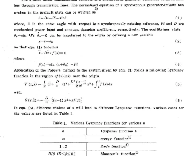
The system under consideration consists of a synchronous generator connected to an infinite bus through transmission lines. The normalized equation of a synchronous generator-infinite bus

2) system in the prefault state can be written as

o+Do=Pi-sino ( 1)

where, iJ is the rotor angle with respect to a synchronously rotating reference, Pi and D are

mechanical power input and constant damping coefficient, respectively. The equilibrium state

iJ0=sin-1Pi, ilo= 0 can be transferred to the origin by defining a new variable x=il-ilo

so that eqn. (1) becomes

x+Dx+f(x)=O where

f(x)=sin (x+ilo) -Pi

(2)

( 3)

(4) Application of the Popov's method to the system given by eqn. (3) yields a following Lyapunov function in the region xf (x) 2 0 near the origin.

· 1 · D D2 _(n-1)

Jx

V(x,x) =--zCx+

n

x)2₊ 2 n2 x2+ /Cx)dx ( 5) with . . D

l

V(x,x)==-n (n-1) x2+xf(x) ( 6)

In eqn. (5), different choices of n will lead to different Lyapunov functions. Various cases for

the value. n are listed in Table 1.

Table 1. Various Lyapunov functions for various n

n Lyapunov function V

oo energy function3)

1 , 2 Rao's function4)

D/p (D:S.,p:S-,0) Mansour's function 5)

1 +Da Pai's function2)

To determine the stability region it is necessary to calculate, first, the unstable equilibrium

state closest to the stable equilibrium state. Then, the critical value Vc of the Lyapunov function

V, which describes the stability boundary, is obtained by substituting such unstable equilibrium

(4)

- - 1 1=00 ---II=-! - - - n=l 0.5 0 0.5 1.0

_,-/·-i

-0.5

:__,_J

--

----

-

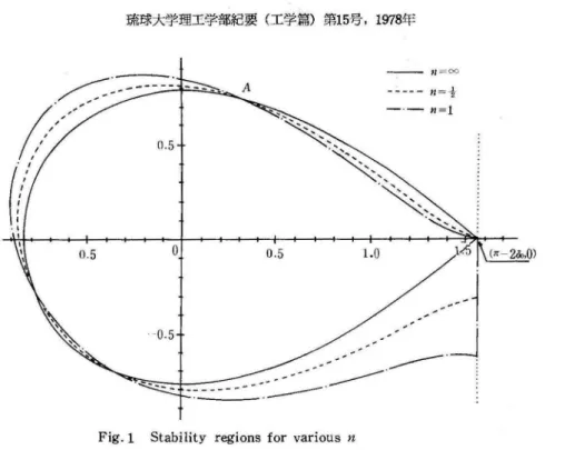
---Fig. 1 Stability regions for various n

Fig. 1 shows the stability regions obtained for the admissible values of n. The system parameters are given as M=l, D=0.2and ilo=45°.

The surface V=Vc passing through the unstable equilibrium state, together with the part of the plane perpendicular to the x-axis with negative x, gives a stability region. An intersecting point A in Fig. 1 is calculated by equalizing two stability boundaries, which are arbitrarily chosen in the limited range of n. Thus, the point A always exists on a curved line

(7) where,

Xc= " - 2oo (8)

Although only three curves are illustrated in Fig. 1, the other stability boundaries depending upon the value of n exist between curves (i) and (ii). When n is infinite. the obtained Lyapunov function corresponds to Gless's function3)and the Lyapunov function (energy function) which is constructed by the authors' method is of this type.

If a system disturbance occurs on a transmission line, the solution trajectory generally lies in the first or third quadrant. Hence, the energy function is often superior to the other Lyapunov functions.

3. Single-machine system with velocity governor

3. 1 Stability region

In this case, the swing equation for the prefault condition is given by2)

;:1 +D~1

+x2--!-j(x1)= 0

x2=gx1-ax2

where,

(5)

108 Transient Stability Regions of Power Systems /Cx1)=sin (x1+oo) -Pi

The additional state variable x2 corresponds to the governor power, while g(=0.1) and a(=0.002) are the parameters of the governor, which is approximated by a single time constant.

According to the previous paperY the system equation (9) is rearranged in the

form

(

! :

J

::

+

l

-

D

0

~

[

~

1

) + [

f

Cx1) ) = [ 0 ) g 1 ₁ x 2 ax2 0 (10)

A modified system obtained by multiplying both members of eqn. (10) by 2 x 2 nons;ngular matrix Q is considered; that is

[

Q11 Q12)f['1

Q21 Q22 .

l

0

o

\

~1

1 + r D

o

)

[

~1

l

+ r/(X1))

l

₌

l

o

J

0

J

x 2 J \- g 1 x 2 \ ax2

f

,

0 The generalized momentum P(x,.i:) and the generalized potential force F(x) become

P (x,x) [ ::: ::: ] [

~

:

)[~:

J

F (x) = [ :::

:::

I

[

/~

::)

J

For a line integral of eqn. (12) to be independent of the path of integration, we obtain

Q21 0

Q12

In consideration of the above relation, the Rayleigh dissipation function W(.i:) is

W (x) =

t

(x1

~2)

[ Qu Q12 ) [ D 0

~

('

~1

J

Q21 Q22 - g 1 ) X2

(D+ : ) Q11

Q22

In order that W(i-) be a positive semidefinite, the conditions

Q11

>

0 • Q22

>

0

(D+!) Qn q22

-

+!}

qu+gq22j

2

;::::

o

must be satisfied. Eqn. (16) reduces to

__L

lg

+

2

D~

/ 4D

(D+__g_)

·-

-

~

qu :::;; Q22 g2 a .. ·. . · V . , a :::;; i2 ·

f!·

··

+

2D+ v /4D CD+:)

l

Q11 Here, we choose Q22 as Q22 = - 1 -g2

l

g / g

r

a-+ 2 D-v 4D CD+a -)

!

Now, the Lyapunov function becomes

· r

1 • 2 aR 2

v

(x,x) = Qtt L~2 x₁ +

-

-z

x₂

+

r

~:

J

(11) (12) (13) (14) (15) (16) (17) (18) (19)

(6)

where,

R = ; 2

~

!

+ 2

D-v/ 4D

CD+

! )

l

Choosing qu as

1

D

we obtain the Lyapunov function

V ( · 1 • 2 aR 2 1

JX1

f

X,x) = 21JXl -1- -2D X2

+

---rJ

0 (Xt)dxt (20) (21) (22)

On the other hand, another Lyapunov function has been obtained by Pai et al. using Popov's method. In case of using Popov's method, the system equation (9) is rewritten in the form

Xt ₀ ₁ ₀ Xt

+

;

X2 0 -D -1 X2

f

(a)

xa

0 g -a X a X1 (23) a = (1 0 0) X2 X a

Notice here that x1 = x2 and x3 now becomes the state variable corresponding to the governor power.

Using transformation

s

+

a

where,

eqn. (23) reduces to the form

I

~~

j

[.

o

l

?2

= . -(aD+g)

~ = - f(a)

- (a+1D) ) [

~:

j

-

[

~

I

f(a)

ab

~a

g

ll

~:

I

+

aD : g ¢

For the system given by eqn. (25), the Lyapunov function obtained by Pai et a!. is

~ ~T V (x,;,a) = Cx

0

B>

r

~

1

(J

+

--jy-J

0 f(a)da where,

_jf

_

l

(a+D)2

+

1l

g(a+D) 0 2D aD+ g 2D(aD+g) B* = g (a-t-D) g 0 ZD(aD+g) 2D(aD+g) 0 0 _·-_2(aD+g)a ... (24) (25) (26) (27)

(7)

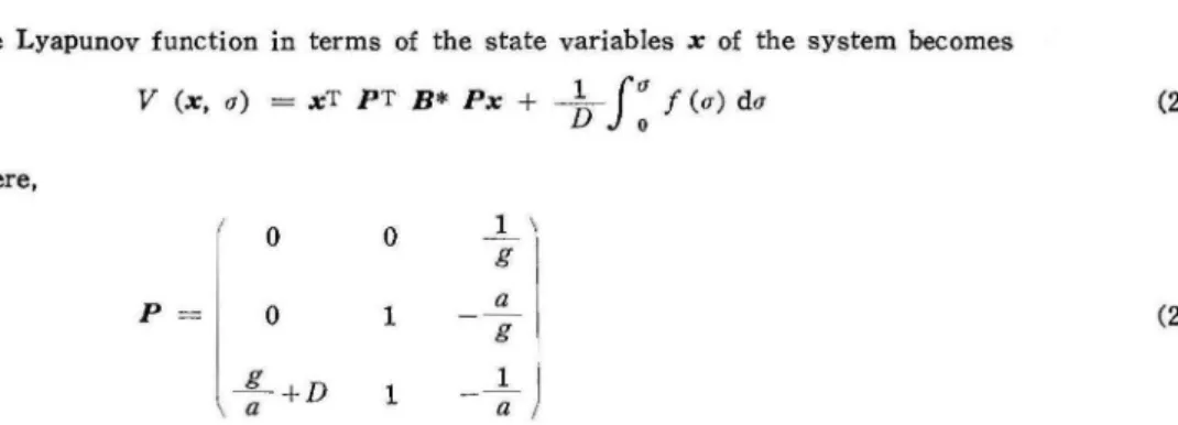
The Lyapunov function in terms of the state variables x of the system becomes

V (x, a) = xT PT B* Px

+

-

1 J:

f

(a) da where, 0 0

l

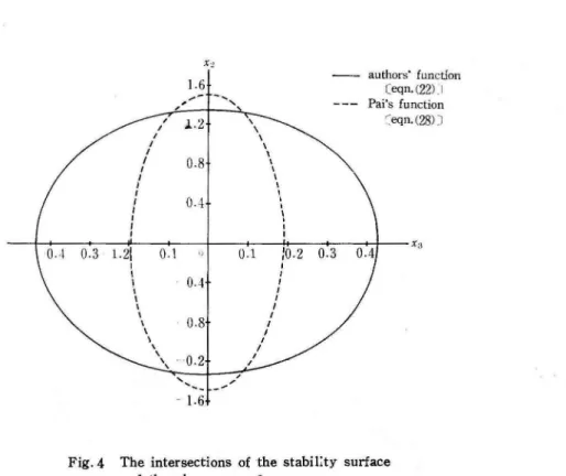
g p ₀ ₁ a g Jf-+D ₁ 1 a a (28) (29)

The stability regions guaranteed by eqn. (22) and (28) are shown in Figs. 2, 3 and 4. The state variables x2 and xa in these figures are corresponding to the variables X1 and x2 in eqn. (22), respectively. The intersections of the plane x3 = 0 of the two Lyapunov functions are sketched in Fig.2. A solid line shows the Lyapunov function {eqn. (22)} given by authors' method and a broken line shows the Lyapunov function {eqn. (28)} given by Popov's method. Figs. 3 and 4 are related to the intersections of the plane x 2 = 0 and x1 = 0, respectively. As shown in these figures, there is no superiority between two Lyapunov functions, being concerned with stability region.

-1.6

X2:

1.6 authors' function ₍_eqn.\22)

----

_{Pai's fun}_c_tion

(eqn.(28)J 0.8

'

_'

\

•

\ \ 0 4 \ \ I I I I 0.4 0 0.4 0.8 1.2 1.6 2.2 2.4 -0.4

Fig. 2 The intersections of the stability surface and the plane xa = 0

(8)

--

---X;\

o.s

0.4 0.3 0.2

---0.1 0 I! . 0.4 0 -0.1 0.2

--- 0.5

---0.4

O)i.--

· t·

:

t

---

---authors' function Ceqn.(22)J Pai's function

---1: eqn. <28))

---.,

...

,.

1.6 2.0 2.4 x,.

Fig. 3 The intersections of the stability surface and the plane x2 = 0

).6 0.8 0.4 0.3 1.21 0.1 I I I ₀_.₄ 0.8

'

' ,_ - 1.6 0.1 10.2

-0.3

authors· function

(eqn.(22U Pai's function

Ceqn.(28)J

Fig. 4 The intersections of the stabil:ty surface and the plane Xt = 0

(9)

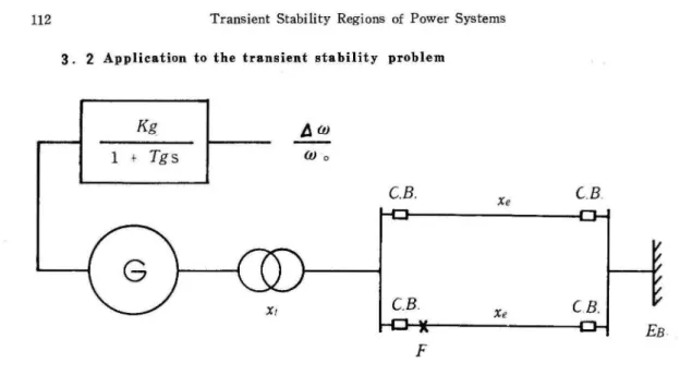
3. 2 Application to the transient stability problem

Kg

1 +

Tgs

W o

C.B

.

_Xe

CB.

C.B

.

Xe

CB.

Es

F

Fig. 5 Power system under consideration

In this section. the authors' method is compared with Popov's method from the point of

view of the critical reclosing time.

A single-machine system connected to an infinite bus taking into account saliency of the

generator is represented by where, Xt + a1 Xt

+

a2 x2 + aaf' Cxt) X2 = bt ~1 - b2 X2 D at=

!vr

J(g

u

--;;-

T

£

Po = Pt sinrio Eq'EB Pt = X12+Xd' ' 1

Tg

0

According to authors' method, the Lyapunov function is obtained as • 2

1 Po

!

cosn0- cos

V(x,x) = 2-xt

-

_Pt aa Xt + as (xt+rlo)

p2

l

COS 2.rlo-COS 2 (XI +i)o)

~

R

'

- ~as + -2

where,

R' = 1

i

(

2 a

t+

b.~

)

-

z./

/~

1

(at+

b

-

1

iz--;-)

(

-

61 '

2' ( . . b2 v b2 J

In order to use Popov's method, eqn. (30) is rewritten in the form

,

;1

1

0 1

~

:: J 0 - at 0 Ct 0 -a2 -c2 0

+

- aa f'(rr) 0 (30) 2 b2 X2 (31)

(10)

( x::t

l

a= (100)

(32)

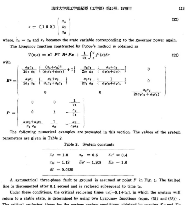
where, Xt = x2 and xs becomes the state variable corresponding to the governor power again. The Lyaqunov function constructed by Popov's method is obtained as

V(x,a) = xT PT B* Px

+

_1_ Ja f'(a)da Ot 0 (33) with 02 Ct (a1+c2) 2 +

1l

a2c1 a1 +c2 0

2a1 as Ca1c2 + a2c1) 2at as a1c2+a2Ct

B*= a2c1 a1+c2 a2c1

1

0

2at as a1c2 +a2c1 2at as a1c2+a2Ct

0 0 _{2(atc2 +}aac2 a2c1) 0 0 1 Ct p 0 1 -~ Ct a1c2+a2cl 1 _~ as c2 a a c2as

The following numerical examples are presented in this section. The values of the system parameters are given in Table 2.

Table 2. System constants

xd = 1.0

XL2 = 1.12 M = 0.0138

Xg

=

0.6

Eq'

=

1.208 En = 1.0

A symmetrical three-phase fault to ground is assumed at point F in Fig. 1. The faulted line :s disconnected after 0.1 second and is reclosed subsequent to time t0 •

Under these conditions, the critical reclosing times <c(=0.1+t0

J,

in which the system will

return to a stable state, is determined by using two Lyapunov functions {eqns. (31) and (33)} . The critical reclosing times for the various system conditions obtained by varying Kg and Tg

are computed. The results are given in Tables 3 and 4, respectively. The results reveal that the Lyapunov function {eqn. (31) } constructed by authors' method is superior to the Lvapunov function {eqn. (33) I obtained by Popov's method.

Table 3. Critical reclosing times for various Kg

"-,.Kg ;

~

-

2.5 5.0 7.5 10.0 12.5 Tr 0.550 0.645 0.785 1.005 1.460 ·-. ---L1 0.535 0.625 0.760 0.980 1.430 -- ·- -L2 Tr L1 L2 0.475 0.560

i

0.695 0.920 1.375 ' Tg=O.l. D""'0.01

step by step method

Lyapunov function constructed by authors' method Lyapunov function constructed by Popov's method

(11)

114 Transient Stability Regions· of Power Systems

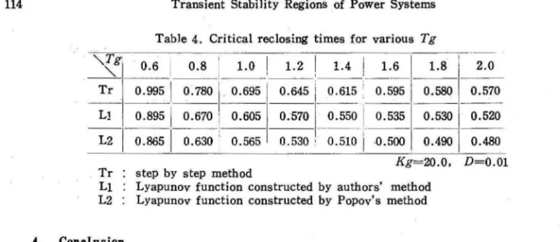
Table 4. Critical reclosing times for various Tg

'"-~T"'g,----,---~---,-~---,--j--,-j ----c~---,~--,...---· _"-_,_1_ 0_._6_ 0.8 1.0 ' 1.2 , _1_.4_: _ _ 1._6 _ __ 1_.8_ 2.0 Tr 0.995 1 0.780 0.695 0.645: 0.615 ; 0.595 0.580 0.570 - - -'1- - --'-- - -- - -- - - - -L! _0.895 ₁_0.670 _0.605 i - - -1-- - -0.8651 0.630 0.565 0.570 0.530

o.sso 1 o.535 o.530 o.52o

-- o.s1o 1 o.5oo o.49o 0.480.

L2 Tr L1 L2 4. Conclusion Kg=20.0, D=0.01 step by step method

Lyapunov function constructed by authors' method Lyapunov function constructed by Popov's method

The Lyapunov function obtained by authors' method has been compared with other Lyapunov functions. In the problem of estimation of critical reclosing time, the proposed function offers better results because of the path of solution trajectory. Hence, one may use the proposed function for the power system stability problems.

Furthermore, since the construction procedure of the authors' Lyapunov function is easy,

such Lyapunov funct:on is considered to be practical.

1

References

Tsuneo Taniguchi and Hayao Miyagi : 'Denryokukeito no Lyapunov Kansu Kosei no Ichihoho',

Trans. of The Institute of Electrical Engineers of Japan, 1977, Voi.97-B, No.5, pp. 271·278

2 :

.

M.A.Pai, M.Ananda Mohan and J.Gopala Rao: 'Power System Transient Stability Regions

Using Popov's Method', IEEE Trans., 1970, Vol.PAS-89, pp. 788·794

3 G.E.Gless: 'Direct Method of Lyapunov Applied to Transient Power System Stability', IEEE

Trans., 1966, Vol.PAS-85. pp. 159-168

4 N.Dharma Rao : 'Routh-Hurwitz Conditions and Lyapunov Methods for the Transient-Stability

Problem', Proc. lEE, 1969, Vol-116, (4), pp. 539-547