IPSS Discussion Paper Series

IPSS Discussion Paper Series

National Institute of Population and Social Security Research Hibiya-Kokusai-Building 6F 2-2-3 Uchisaiwai-Cho

Chiyoda-ku Tokyo, Japan 100-0011 (No.2007-E02)

Household projection 2006/07 in Japan using a micro-simulation model

Tetsuo Fukawa, Ph.D.

(National Institute of Population and Social Security Research)

Oct. 2007

IPSS Discussion Paper Series do not reflect the views of IPSS nor the Ministry of Health, Labor

and Welfare. All responsibilities for those

papers go to the author(s).

Household projection 2006/07 in Japan using a micro-simulation model 12 Oct. 2007

Tetsuo Fukawa

National Institute of Population and Social Security Research

By using a micro-simulation model named INAHSIM, we conducted household projection 2006/07 in Japan for the period of 2005-2050. Concerning the elderly, the model produces such outputs as a) the number of the elderly according to different living situation, b) the number of the elderly by physical condition x living situations, and c) the relative number of parents weighted by the number of brothers and sisters of children. Distribution of the elderly by physical condition and living arrangement is important in considering social support for the elderly, especially long-term care.

1. Introduction

The household is one of the most important statistical bases for policy formulation on health and welfare. Statistical information on households and families is still inadequate, although expanding recently, to understand the dynamic process of formation and dissolu- tion of households and families in a systematic and coordinated way.

Dynamic micro-simulation is one method for household projections, in which the state of individuals is to change stochastically through vital and other events. Quite con- trary to macro simulation, in which population is distributed deterministically and vital events occur to the population as a whole, occurrence and timing of various events in mi- cro simulation are decided stochastically at the individual level. Static micro-simulation models are most frequently used to provide estimates of the immediate distributional im- pact of policy changes. Dynamic micro-simulation models often start from exactly the same cross-section sample surveys as static models. However, the individuals within the original microdata are then progressively moved forward through time; this is achieved by making major life events- such as death, marriage, divorce, fertility, education, labour force participation etc- happen to each individual, in accord with the probabilities of such events happening to real people within a particular country (Harding, 1996).

Dynamic micro-simulation models are widely used in Europe, Australia and North

America for the evaluation and planning of many social policies (Inagaki, 2007). Informa-

tion on each category of population can be tabulated flexibly without changing the main

framework of the simulation. Dynamic micro-simulation method does have some draw-

backs, including difficulties in obtaining the initial population and estimating the transition

probabilities, and existence of sampling errors owing to the use of random numbers. Be-

cause of the consistency and flexibility, however, dynamic micro simulation is considered

to be the most suitable method to observe dynamic evolution of households and families and to forecast their future trends (Fukawa, 1995). While most micro-simulation models developed to date have focused on the household sector, a number have been created which simulate the behaviour of business firms, rather than individuals or households (Harding, 1996).

INAHSIM (Integrated Analytical Model for Household Simulation) is a dynamic mi- cro simulation model, which was first developed in 1984-85 in Japan by using actual ini- tial population derived from a household survey and a set of transition probabilities de- rived from population census, vital statistics and several national sample surveys (Aoi et al, 1986). Among several attempts to improve the simulation model since 1985, a new appli- cation of the model has been made in 1993-94, which we call as 1994 Simulations. Char- acteristic features of 1994 Simulation were: a) the initial population was formed by using the INAHSIM model itself; and b) the dynamic transition of household types was particu- larly focused upon. The 2004 Simulation improved the creation of the Initial Population further and added the physical condition of the elderly in the model. The main purpose of INAHSIM was to prepare projections to get information on the future number and compo- sition of households, and to analyze households and families in terms of dynamic transi- tion of household types, family systems, etc.

Events contained in this model include not only such vital events as birth, death, mar-

riage, divorce, and changes of household situations generated by them, but also separation

from and return to original household, reuniting of widowed or divorced persons to the

parent’s household, and merger of aged parent(s) to the child’s household (Note 1). The

death rate is given by age and sex for those who are less than 65 years old, but it is deter-

mined by transition probability which is given by age, sex, and physical condition for

those who are 65 years old or over. Separation from original household means here that the

married or unmarried individual separates from his/her original household temporarily and

newly forms a one-person household. Return to original household means just the opposite

process of separation. We employ four kinds of household merger: (a) Co-resident rate of

adult child with parents upon marriage, (b) Reuniting rate of adult child to the parent’s

household upon becoming widowed, (c) Reuniting rate of adult child to the parent’s

household upon divorce, and (d) merger rate of aged parent(s) with child generation by

marital status, average age and physical condition of aged parent(s). The operation of each

event is done once a year, and the order of the operation is as follows: marriage, birth,

death, divorce, separation, return, and merger of aged parents. Reuniting of widowed or

divorced to the parent’s household is included in the operation of death or divorce respec-

tively.

2. Framework of the 2006/07 Simulation

Observing the basic framework of 2004 Simulation, this 2006/07 Simulation has the fol- lowing characteristics: a) the initial population was formed by using INAHSIM model it- self; b) the physical condition of the elderly is related to the data of the Long-term Care Insurance (LCI); c) institutions are included in the model as a possible option for the eld- erly to move to. Whether a person moves to an institution or not depends on age, marital status, and physical condition of the elderly.

(1) Initial Population

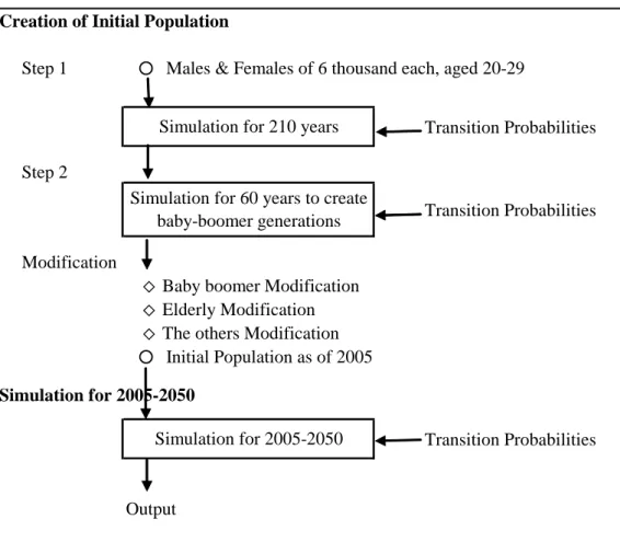
Preparation of initial population was done by three steps as shown in Fig. 1. First, a group of males and females of 6,000 each, aged 20-29 according to age distribution in 2005, was created and thrown into the model. A simulation was executed for 210 years in order to obtain a stable state, using a set of transition probabilities prepared for this process. Next in

Fig. 1 Flow chart of INAHSIM 2006/07 Simulation Creation of Initial Population

Step 1 　 ○ 　Males & Females of 6 thousand each, aged 20-29

Transition Probabilities Step 2

Transition Probabilities Modification

　 ◇ Baby boomer Modification 　 ◇ Elderly Modification 　 ^◇ The others Modification 　 ○ 　Initial Population as of 2005 Simulation for 2005-2050

Transition Probabilities

Output

Simulation for 210 years

Simulation for 60 years to create baby-boomer generations

Simulation for 2005-2050

Step 2, baby-boomer generations were created using a specific set of transition probabili-

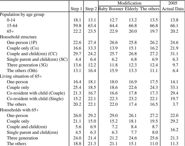
ties. The final state of this second step, which was shown at the “Step 2” column of Table

1, was subject to modifications. Three modifications were done at this step in order to ob- tain such an initial population as reflected the age and household structure of the actual population in 2005. Baby-boomer modification was still necessary to create baby-boom cohorts in the model. The other two modifications were done to produce more suitable ini- tial population in terms of age structure and household composition. Through these modi- fications, the initial population consisted of 85,415 individuals in 29,683 households. Ob- tained initial population was fairly good in general (Table 1). However, there was still a considerable discrepancy in the living situation of the elderly between the initial popula- tion and actual data in 2005. Throughout the simulation, the initial population was fixed.

Table 1 Creation of Initial Population for 2005

（In ％）

2005 Step 1 Step 2 Baby Boomer Elderly The others Actual Data Population by age group

0-14 18.1 13.1 12.7 13.2 13.5 13.8

15-64 59.8 63.4 64.4 66.8 66.8 66.1

65+ 22.2 23.5 22.9 20.0 19.7 20.2

Household structure

One-person (1P) 22.6 27.4 26.6 25.8 26.2 24.6

Couple only (Co) 16.6 13.3 13.9 15.1 16.2 21.9

Couple and child(ren) (CC) 29.7 24.2 25.7 26.8 27.2 31.1

Single parent and child(ren) (SC) 4.4 6.4 6.2 6.8 6.9 6.3

Three generation (3G) 13.6 12.2 11.8 12.3 12.4 9.7

The others (Oth) 13.1 16.4 15.9 13.3 11.1 6.4

Living situation of 65+

One-person 16.4 18.1 18.0 16.9 17.5 14.1

Couple only 25.4 18.5 18.6 22.6 24.3 33.1

Co-resident with child (Couple) 21.3 16.7 16.6 17.8 17.3 29.4 Co-resident with child (Single) 15.2 22.1 22.3 23.2 22.1 19.7

The others 20.2 22.1 22.0 17.4 16.5 3.7

Households with 65+

One-person 26.0 29.2 29.0 26.1 27.2 22.0

Couple only 21.1 15.0 15.2 18.1 19.5 29.2

Couple and child(ren) 5.6 6.9 7.2 8.4 8.7

Single parent and child(ren) 4.5 6.3 6.3 7.7 8.0

Three generation 24.0 21.4 21.2 24.6 25.6 21.3

The others 18.8 21.3 21.1 15.1 11.0 11.3

Modification

16.2

(2) Transition Probabilities

Various transition probabilities are used in the model (Note 2). The total fertility rate was

assumed to remain around 1.28 for S1 and around 1.44 for S2 throughout the simulation

period, and results from S1 are used in the next section. Contrary to the fertility rate, the

death rate is assumed to decline gradually, and life expectancy at birth will be 81.8 years

for males and 88.4 years for females in 2050. Although we did not apply it this time, the

family system can be expressed by a set of three probabilities in this model: co-resident rate of adult child with parent upon marriage, reuniting rate of divorced or widowed per- sons to his/her parent’s household, and merger rate of aged parent(s) to the child’s house- holds.

The physical condition of the elderly aged 65 or over is classified into 4 levels as fol- lows:

Level 0: No disability and completely independent;

Level 1: With some disability but basically independent;

Level 2: Slightly or moderately dependent; and Level 3: Heavily dependent.

Levels 2 and 3 correspond to the eligible persons of the LCI, and Level 3 corresponds to care need levels 4 and 5 in particular. The merger rate of aged parent(s) changes according to age, marital status and physical conditions (Note 3). As institutions are incorporated in the model this time, we assume that an aged person tends to move to an institution as his/her physical condition deteriorates (Note 4).

3. Results of the 2006/07 Simulation 3.1 Basic Results

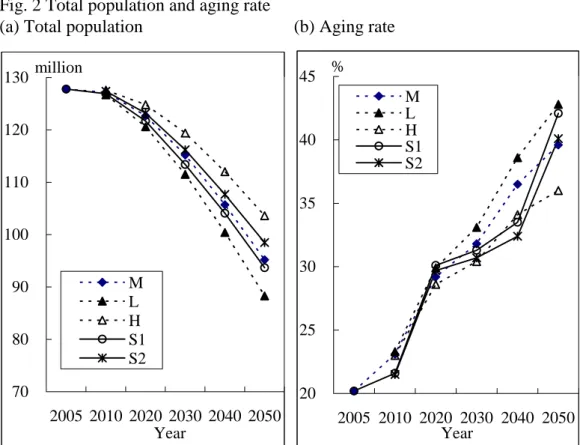
According to the 2006/07 simulations, the Japanese total population started decreasing from 2005, while aging of the population will continue until 2050 (Fig. 2). Total popula- tion and aging rate (the proportion of those who are 65 years old or over to the total popu- lation) in future years are in line with the result of the latest population projection pub- lished in December 2006.

Although the number of total households will start decreasing from 2005 same as the total population, the numbers of both households headed by the elderly (65+) and house- holds with the elderly (65+) will increase until 2020 (Table 2). Table 2 also shows the dis- tribution of children aged 0-14 by household type. The number of three-generation house- holds is anticipated to decrease in future, and the number of children living in the three-generation households will decrease accordingly.

Fig. 2 Total population and aging rate

(a) Total population (b) Aging rate

Note: M, L, H mean middle, low, and high scenario of the Population Projection as of December 2006 respectively.

70 80 90 100 110 120 130

2005 2010 2020 2030 2040 2050 Year

million

M L H S1 S2

20 25 30 35 40 45

2005 2010 2020 2030 2040 2050 Year

%

M L H S1 S2

Table 2 Future Population and Households

(In million, %)

Total Elderly

CC SC 3G

2000 126.9 14.6 68.1 17.4 7.1 22.0 45.5 15.6 2005 127.8 13.8 66.1 20.2 9.1 25.7 48.0 13.8 a 18.5

2010 126.9 13.7 64.7 21.6 11.2 27.5 46.7 17.6 20.9 53.7 4.2 29.7 2020 121.7 11.5 58.4 30.1 13.6 36.6 45.7 22.5 25.4 53.0 4.1 30.7 2030 113.4 9.6 59.1 31.3 20.7 35.5 43.6 22.0 24.8 51.9 3.9 31.6 2040 104.1 10.1 56.4 33.5 20.6 34.9 40.5 21.0 23.8 49.4 4.6 31.5 2050 93.7 9.1 48.8 42.1 22.6 39.4 37.3 23.1 25.3 49.5 4.6 30.7 a 2004

Elderly in this table means those who are 65 years old or over.

Distri. of children (0-14) by household type (%)

Population

65+ 75+

Age Structure (%)

Number of Households Total

Headed by the Elderly

With the Elderly 0-14 15-64

3.2 Projections on the elderly

Table 3 shows the living situation of the elderly (65+). In 2004, among the elderly popula-

tion, 14.7 percent live in one-person households, 36.0 percent in couple-only households

and 45.5 percent live with the child generation. According to the simulation, the proportion of one-person households will increase and the proportions of both couple-only house- holds and co-resident households will decrease. The proportion of those elderly who stay in institutions will steadily increase until 2040.

Table 3 Living situation of the elderly (65+)

（ In ％）

1P Co 1P Co 1P Co

a b c d a b c d a b c d

2004 14.7 36.0 8.2 46.5 19.6 28.0

2010 18.4 21.9 6.3 8.5 15.1 9.0 2.6 14.7 28.0 7.8 3.8 20.9 4.3 21.4 17.0 5.1 12.2 10.4 12.7 2020 16.7 19.8 6.3 6.1 17.3 8.9 2.9 13.7 24.2 7.6 2.9 21.7 4.5 19.1 16.2 5.4 8.8 13.8 12.4 2030 17.6 16.4 6.1 6.5 14.6 10.5 4.4 15.2 20.9 7.4 3.3 18.9 5.4 19.5 12.9 5.0 9.0 11.3 14.5 2040 17.2 14.6 5.4 6.5 12.5 11.3 5.6 14.9 18.8 6.8 3.1 16.8 6.0 19.0 11.3 4.3 9.2 9.2 15.4 2050 17.5 16.3 5.0 5.5 12.5 8.9 4.9 15.8 19.2 5.9 2.8 16.4 4.9 18.9 14.0 4.4 7.6 9.3 12.2 Note: Co-resident with child

Co-resident with child

Co-resident with child

Single Child

Insti- tution Co-resident with

child

c d Elderly

Couple Single

Couple a b Year

27.5 21.0

23.6 21.9 18.4 23.2

Total Male Female

The living situation of the elderly is rather different between males and females as shown in Fig. 3. Reflecting the difference in death rates, the proportion of one-person households is higher and that of couple-only households is lower for females than males.

The number of female elderly staying in institutions is higher than that of male elderly.

However the proportion of those who stay in institutions is rather similar between males and females.

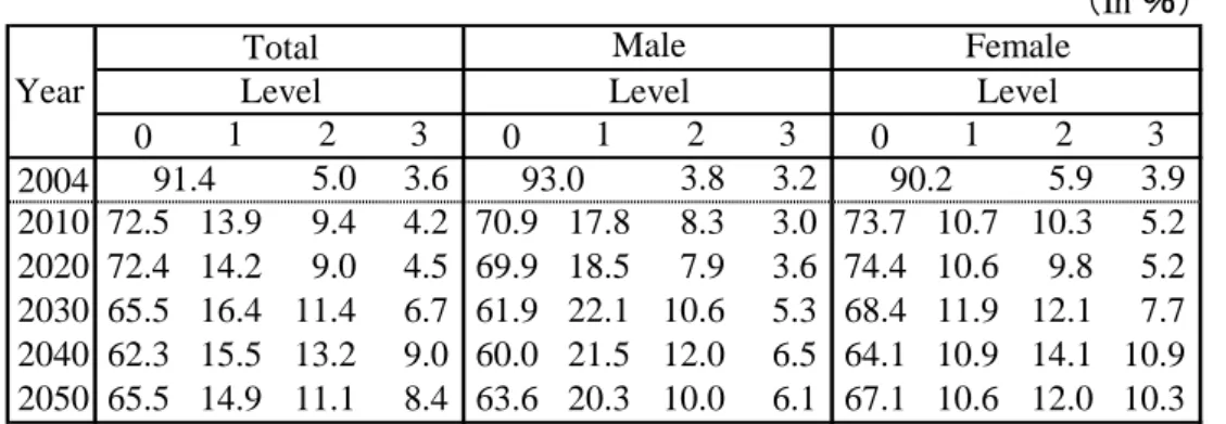
Baseline data for the physical condition of the elderly in 2004 are obtained from the

national sample survey conducted by the Ministry of Health, Labour and Welfare as shown

in Table 4. The proportion of those elderly whose physical condition is in level 3 will

steadily increase especially among females.

Fig. 3 Living situation of the elderly by age group and sex

a) One-person b) Couple-only

c) Co-resident with child generation d) Institution 10

15 20 25 30 35

2010 2020 2030 2040 2050 Year

% Male

Female

●

65+

＊ 75+

5.0 10.0 15.0 20.0 25.0 30.0

2010 2020 2030 2040 2050 Year

%

25.0 30.0 35.0 40.0 45.0

2010 2020 2030 2040 2050 Year

%

0.0 5.0 10.0 15.0 20.0

2010 2020 2030 2040 2050 Year

%

Relative number of parents weighted by the number of brothers and sisters of chil- dren is obtained from the model as follows (Fukawa, 2005):

R(y) = Relative number of parents according to age group of children (y);

n = number of brothers and sisters of children;

F(y) = Σ F(y, n), where F(y, n) = Number of children at age group of y with n brothers n

and/or sisters;

G(y) =ΣG(y, n)/ n, where G(y, n) = Number of parents with children at age group of y n

and n brothers and/or sisters;

R(y) = G(y) / F(y)

Table 4 Distribution of the elderly (65+) by physical condition level

（In ％）

0 1 2 3 0 1 2 3 0 1 2 3

2004 5.0 3.6 3.8 3.2 5.9 3.9

2010 72.5 13.9 9.4 4.2 70.9 17.8 8.3 3.0 73.7 10.7 10.3 5.2 2020 72.4 14.2 9.0 4.5 69.9 18.5 7.9 3.6 74.4 10.6 9.8 5.2 2030 65.5 16.4 11.4 6.7 61.9 22.1 10.6 5.3 68.4 11.9 12.1 7.7 2040 62.3 15.5 13.2 9.0 60.0 21.5 12.0 6.5 64.1 10.9 14.1 10.9 2050 65.5 14.9 11.1 8.4 63.6 20.3 10.0 6.1 67.1 10.6 12.0 10.3 Note: Physical condition level

0: No disability and completely independent 1: With some disability but independent 2: Slightly or moderately dependent 3: Heavily dependent

Year

Male

Level Level

91.4 93.0 90.2

Female Total

Level

Fig. 4 shows the results for the years 2010, 2030, and 2050. As low fertility continues and life expectancy prolongs, the relative weight of parents to adult children will increase remarkably in the future. The relative weight of mothers is higher than that of fathers re- flecting the difference of death rate by sex.

Fig. 4 Relative number of parents according to age group of children

Relative number of parents

0.0 0.2 0.4 0.6 0.8 1.0 1.2 1.4 1.6

0-4 5-9 10- 14

15- 19

20- 25- 30- 35- 40- 45- 50- 55- 60- 64

65- 69

70- 74 Age group of children

2010

father

mother

2030

2050

3.3 Dynamic Transition of Households

Table 5 shows one-year transition matrix by household type for the years 2009-2010 and 2049-2050. As the net increase/decrease in the number of total households is the difference between newly formed households and dissolved households during a year, the number of households with structural change can be greater even if the net increase/decrease is small.

From 2009 to 2010, 2,092,000 households are estimated to be newly formed and 2,148,000 dissolved, resulting in 56,000 as net decrease. During 2009-2010, 41,396,000 households will remain in the same household structure, and 3,236,000 households will change their household structure. Therefore, the total number of households changed (i.e.

newly formed, dissolved or transformed the household structure) will be 7,476,000, which is more than 130 times the net decrease.

Table 5 One-year transition matrix by household type

2009-2010 （46,780→46,723） (In thousand)

Total 46,780 10,887 7,908 12,385 3,141 5,606 6,797 2,148

One-person (IP) 10,960 8,664 86 34 136 3 53 1,983

Couple-only (Co) 7,851 236 7,022 451 15 0 61 66

Couple and child (ren) (CC) 12,534 5 462 11,606 178 95 175 13 Single parent and child (ren) (SC) 3,218 257 0 27 2,745 15 110 65

Three-generation (3G) 5,643 0 6 92 16 5,270 259 0

The others (Oth) 6,574 118 44 40 39 223 6,089 21

Newly formed - 1,607 288 134 13 0 50 -

2049-2050 （37,616→37,280） (In thousand)

Total 37,616 10,423 5,916 6,345 2,541 3,550 8,506 1,455

One-person (IP) 10,415 8,924 40 13 84 2 27 1,324

Couple-only (Co) 5,979 192 5,457 223 10 2 44 52

Couple and child (ren) (CC) 6,438 6 221 5,957 99 57 79 19 Single parent and child (ren) (SC) 2,619 228 0 18 2,292 2 39 40

Three-generation (3G) 3,643 2 3 47 15 3,357 220 2

The others (Oth) 8,522 157 92 21 32 131 8,069 19

Newly formed - 913 102 66 10 0 27 -

Number

in 2009 Oth

1P

Disso- lved Number in 2050

Co CC SC 3G Oth

Household type

Household type

Disso- lved Number in 2010

1P Co CC SC 3G

Number in 2049

As shown in Table 5, one-person households will increase from 10,960,000 in 2009

to 10,887,000 in 2010: 1,607,000 will be newly formed, 1,983,000 will be dissolved by

death, return, merger of the aged, etc., 236,000 will change from couple-only households

to one-person households by divorce or death of the spouse, and 257,000 will change from

“single parent and child(ren)” households. Couple-only households are also relatively un- stable. Out of 7,851,000 of couple-only households, 7,022,000 will remain, 462,000 will change from couple and child(ren) households to couple-only households, and 288,000 will be newly formed by marriage during the year 2009-2010.

There are some frequent patterns in streams of change according to Table 5.

One-person households have a strong tendency to change: to be dissolved, to be newly formed, to change from couple-only households or single parent and child(ren) households.

Couple-only households are newly formed by marriage, change to and from couple and child(ren) households, etc. Single parent and child(ren) households tend to change to one-person households by their children’s marriage or independence, and some transfer to the other categories of household by co-residence with their married children.

The stability of each household type is measured by the yearly transition rate, which is calculated by 1 – (Number of continued households) / (Average number of households).

The average number of total households during 2009-2010 will be 46,752,000, and the number of continued households will be 41,396,000. Therefore, annual rate of transfer for the total households during 2009-2010 will be 11.5 percent, and this means that the ex- pected duration of household newly formed during 2009-2010 will be 8.7 years (Table 6).

The expected duration of one-person households and couple-only households has a ten- dency to increase over time, but three-generation households have the opposite tendency in expected duration. However, we need a careful examination of all transition probabili- ties employed to lead any concrete interpretation out of this table.

Table 6 Yearly transition rate and expected duration by household type

Total 46,752 11.5 8.7 40,230 9.1 11.0

One-person 10,924 20.7 4.8 11,799 14.3 7.0

Couple-only 7,880 10.9 9.2 6,903 8.2 12.1

Couple and child (ren) 12,460 6.9 14.6 7,559 6.8 14.7

Single parent and child (ren) 3,180 13.7 7.3 2,888 11.2 9.0

Three-generation 5,625 6.3 15.9 2,370 6.7 15.0

The others 6,686 8.9 11.2 8,712 5.2 19.1

Household type

From 2009 to 2010 From 2049 to 2050 Average N.

of households (Thousand)

Yearly transition

rate (%)

Expected duration (Year)

Average N.

of households (Thousand)

Yearly transition

rate (%)

Expected duration

(Year)

4. Discussion

INAHSIM was first developed in 1984-85 by a multi-disciplinary research group. In 1994

Simulation, the initial population of the model was prepared by using the simulation model

itself. It has been confirmed that INAHSIM is applicable when the initial population is not available from census or national household surveys, and all problems caused by the initial population without the information about family members residing outside of the household will be avoided though creating an initial population by using the simulation model itself (Fukawa, 1995). In 2004 Simulation, the creation process of the initial population was im- proved and physical condition of the elderly was introduced in the model. In this paper, based on the 2004 Simulation, the physical condition of the elderly is related to the data of the Long-term Care Insurance and we incorporated institutions in the model for the first time.

The INAHSIM provides us, among others, with information on the dynamic transi- tion of household types, the effects of family systems on the number and structure of households, and household situations of individuals with specific attributes. The household situation of the children is basic information for a well-defined child care support policy.

The dynamic transition of households is always a good example of the predominant fea- tures of micro-simulation model. By changing the starting year of the simulation, INAHSIM is useful for both historical analysis and future projection of households and families (Fukawa, 1995). While dynamic models typically do capture some types of be- havioural change, they face problems (like static models) when attempting to incorporate either behavioural change in response to government policy changes or second round ef- fects because they do not necessarily allow changes in behaviour initiated by government policy change (Harding, 1996).

It turned out to be very important to connect the living situation and physical condi- tion of the elderly. Expenditure of the LCI in 2004 was 6.0 trillion yen, 1.2 percent of GDP, providing benefits to 3.1 million people equivalent to 12.3 percent of the elderly. Due to aging of the population, the dependent elderly will increase rapidly in the future as shown in Table 4, and the distribution of the elderly by living situation and physical condition has a direct implication on the future expenditure of the LCI. A weighted parent-child ratio is an index of elderly care, and the usefulness of such an index increases through incorporat- ing the physical condition of the elderly.

From the INAHSIM, we can obtain a population-household projection in a coherent

manner as well as dynamic statistics which are difficult to obtain from static surveys or

macro simulation. If we construct a pertinent initial population and improve accuracy of

transition probabilities, then we can extract useful information from the INAHSIM which is

only available from micro-simulation. The structure of INAHSIM is flexible enough to

change output tables without changing main framework of the simulation, and to improve

output information by putting additional simulation variables (Fukawa, 1995). Transition

probabilities are able to be changed annually. In this model, the family system is expressed

by a set of probabilities, and by changing these variables, the model can express different

family systems. In order to analyze the family lifecycle, it is necessary to improve the ac- curacy of various transition probabilities on household mergers. By adding place of dwell- ing, housing and employment situation in the model, we can improve the usefulness of the model remarkably. Inagaki (2005) added employment situation in the model, and analyzed the effects of recent increase in non-regular workers to the future fertility and household situation.

Notes:

(Note 1) Occurrence of each event is based on the Monte-Carlo method: that is if and only if a random number generated by the computer for each event is equal to or smaller than the probability given, the event is allowed to occur. When an event is decided to occur, all nec- essary procedures will be done step by step to simulate the changing actual society.

(Note 2) Transition Probabilities

Birth: Birth rate: age of mother and birth order

Sex ratio at Birth: 105.5 males for 100 females Death: Death rate: age and sex for 0-64 years old

Transition probability: age, sex and physical condition for 65+

Marriage: First marriage rate: age and sex Re-marriage rate: age and sex Divorce: Divorce rate by duration of marriage

Probability of husband leaving household upon divorce: 0.6939 Separation & Return: Separation rate: age, sex and marital status

Return rate: age, sex and marital status Household Merger:

Co-resident rate of adult child with parents upon marriage

bridegroom's = 0.40901, bride's = 0.17647 (no brothers), 0.02373 (otherwise) Reuniting rate of adult child to the parent's household upon becoming widowed: 0.3 Reuniting rate of adult child to the parent's household upon divorce: 0.43 (male), 0.35

(female)

Merger rate of aged parent(s) with child generation: marital status, average age of aged parent(s), and physical condition

(Note 3) Standard merger rate of aged parent(s), U, changes according to age and marital status: Single male 65: 0.015, 100: 0.207; Single female 65: 0.015, 100: 0.123; Couple 65:

0, 100: 0.05. Standard rate U is modified according to physical conditions as follows:

Physical condition

0 1 2 3

Single ^× 0.8 × 1.0 × 1.5 Always 1.0

Couple ^× 0.5 ^× 0.5 ^× 0.7 ^× 1.0

(Note 4) The following patterns are assumed concerning the probability of the elderly to move into institutions (number shows physical condition level):

Single 2: Merge to child generation, or move to institution Single 3: Always move to institution

＊ : Do not move to institution

a): merge to child generation, otherwise [2] moves to institution b): [3] always moves to institution

+: Both move to institution

References

Aoi, Kazuo, Yoichi Okazaki, Tetsuo Fukawa, Kyo Hanada et al. (1986). Household projec- tion by INAHSIM: A comprehensive approach. Life Span vol. 6. (in Japanese)

Fukawa, Tetsuo. (1995). Future Trends of Japanese Households through Micro simulation Model- An application of INAHSIM. The Journal of Population Studies, 18, 13-27.

Fukawa, Tetsuo. (2005). Household Simulation 2004 through INAHSIM. The Journal of Population Studies, 36, 1-12. (in Japanese)

Hammel, D. A. et al. (1976). The SOCSIM Demographic Sociological Micro Simulation Programme: Operating Manual, Research Series, No. 7, University of California, In- stitute of International Studies, Berkly.

Hanada, Kyo, Mitsuru Hata and Ryo Sato. (1980). Financial Projection of Public Pension by Micro Simulation Model in Japan. Nenkin-Kenkyu No. 8. (in Japanese)

Hanada, Kyo, Tetsuya Ito and Shigemi Kono. (1988). The Future of Japanese Families: A Micro Simulation Study. IUSSP Seminar on Theories of Family Change, Tokyo, No- vember 29-December 2, 1988.

Harding, Ann. (1996). Introduction and Overview. in Harding (ed.), Microsimulation and Public Policy, North-Holland.

Havema, R. H. and Hollenbeck, K. ed. (1980). Microeconomic Simulation Models for Pub- lic Policy Analysis, Academic Press.

Inagaki, Seiichi. (1986). An Analytical Model on Household and Family via Micro Simula- tion (INAHSIM). Blletin of the Institute of Actuaries of Japan, 39, 89-188. (in Japa-

Couple: 0 1 2 3

0 1 2 3

＊

＊

＊ b)

＊

＊ a) b)

＊ a) + +

b)

b)

+

+

nese)

Inagaki, Seiichi. (2005). Projections of the Japanese Socioeconomic Structure Using a Mi- crosimulation Model (INAHSIM). IPSS Discussion Paper Series (No.2005-03).

Inagaki, Seiichi. (2007). Analysis of Future Social-Demographic Structure of Japan –Projection Using a Dynamic Microsimulation Model (INAHSIM). (in Japanese) Inoue, Shunichi. (1977). Choice of Policy Measure to Affect Fertility: A Computer Mi-

cro-Simulation Study, Population Bulletin of the United Nations, No. 10.

Menken, Jane A. (1978). Current Status of Demographic Models, Population Bulletin of the United States, No. 9.

National Institute of Population and Social Security Research. (2004). Household Projec- tions for Japan: 2001-2025. Tokyo, Health and welfare Statistics Association. (in Japanese)

National Institute of Population and Social Security Research. (2007). Population Projec- tions for Japan: 2006-2055. Population Research Series 315. (in Japanese)

Orcutt, G., Caldwell, S. and Wertheimer, R. F. (1976). Policy Exploration Through Micro- analytic Simulation, The Urban Institute, Washington D. C.

Wachter, K. W. (1978). Statistical Studies of Historical Social structure, Academic Press.

IPSS Discussion Paper Series（English）

No Author Title Date

2007-01 Takanobu Kyogoku In Search of New Socio-Economic Theory on Social Security

May 2007

2005-07 Aya Abe Empirical Analysis of Relative Deprivation and Poverty in Japan

March, 2006

2005-04 Takashi Oshio and Satoshi Shimizutani

The impact of social security on income, poverty, and health of the elderly in Japan

October 2005

2005-03 Seiichi INAGAKI Projections of the Japanese Socioeconomic Structure Using a Microsimulation Model (INAHSIM)

October 2005