A degenerate singularity generating geometric Lorenz attractors

A degenerate singularity generating geometric Lorenz attractors

Freddy Dumortier

Departement Wiskunde, Limburgs Universitair Centrum Universitaire Campus, B-3590 Diepenbeek, BELGIUM

Hiroshi Kokubu

Department of Mathematics, Faculty of Science, Kyoto University, Kyoto 606-01, JAPAN

and Hiroe Oka

Department of Applied Mathematics and Informatics Faculty of Science and Technology, Ryukoku University

Seta, Otsu 520-21, JAPAN January 20, 1995

Abstract

A degenerate vector eld singularity in IR³ can generate a geometric Lorenz attractor in an arbitrarily small unfolding of it. This enables us to detect Lorenz-like chaos in some families of vector elds, merely by performing normal form calculations of order 3.

1

1 Introduction

The local bifurcation theory for vector elds deals with changes of dynamical structure of a vector eld germ under perturbation. The Hartman-Grobman Theorem Palis and de Melo 1982] tells us that a hyperbolic vector eld singu- larity is locally structurally stable, namely, it has the same dynamical structure as a nearby vector eld singularity does | no bifurcation occurs after pertur- bation. Singularities other than hyperbolic ones, on the contrary, do undergo bifurcations and hence they are called \degenerate singularities".

Bifurcations appearing from such degenerate singularities strongly depend on the singularity itself. A singularity having a simple zero eigenvalue in its linear part as well as non-degenerate higher order terms generates a pair of equilibria after perturbation, which is called the saddle-node bifurcation. A sin- gularity having one pair of pure imaginary eigenvalues in the linear part together with non-degenerate nonlinear terms gives rise to a limit cycle bifurcating o from the singularity, which is known as the Andronov-Hopf bifurcation (e.g.

Dumortier 1991]). More complicated bifurcations occur from more degenerate singularities, by which a homoclinic orbit, an invariant torus, or chaotic dy- namics can be generated Guckenheimer and Holmes 1983]. Those degenerate singularities have been studied extensively but many important cases are still left for further investigation.

The purpose of this paper is to show that even a strange attractor can be generated from certain degenerate singularities. Namely, we shall prove the following:

Theorem 1.1.

Let v be a vector eld singularity in IR³ whose 3-jet is given by y @@x ^;x³ @

@y ⁺x² @

@z ⁽⁽xyz)²IR³):

Then there exists an arbitrarily small unfolding of the singularity which contains a geometric Lorenz attractor.

Here a geometric Lorenz attractor (Guckenheimer 1973], Guckenheimer and Williams 1979], Williams 1979]) is a mathematically formulated geomet- ric model of the Lorenz attractor (Lorenz 1963]) which is a strange attractor observed by computer simulation of the following ordinary dierential equation:

x_ =(y^;x) y_ =rx^;y^;xz

z_ =^;bz+xy ⁽¹:1) 2

with = 10r = 28b = ⁸³. The above theorem shows that an unfolding of cer- tain degenerate singularities contains a (miniature of) strange attractor which satises the denition of geometric Lorenz attractors given by Guckenheimer and Williams. More precise statement is given in ^x3. Important is that the ex- istence of such a geometric Lorenz attractor in an unfolding can be veried by a simple normal form calculation of equations up to terms of order 3, and therefore it may be possible to use the result as a criterion for the existence of \Lorenz-like chaos" in given systems | in a similar way as the Andronov- Hopf bifurcation theorem has been used for a criterion to detect an oscillatory motion.

For the rest of this paper, we shall give a proof of the above theorem. In

x2, the singularity is heuristically introduced from the original Lorenz equation (1.1) according to Ushiki, Oka and Kokubu 1984], and in ^x3, the main result is stated in a more precise manner by specifying the necessary unfolding terms. In

x4, we shall give several additional properties of the singularity. ^x5 is devoted to a preliminary rescaling argument by which the unfolding is reduced to a cer- tain type of homoclinic bifurcation problem. This particular homoclinic orbit is called an `inclination-ip' homoclinic orbit studied by Yanagida 1987], Kisaka, Kokubu and Oka 1992], and Rychlik 1990]. The precise denition will be given in ^x6 together with a theorem due to Rychlik 1990] which plays an important role for our result: He showed that a symmetric pair of such inclination-ip homoclinic orbits with a certain eigenvalue condition can generate a geometric Lorenz attractor in its perturbation. In order to apply Rychlik's theorem to our case, we need to perturb our system in order to verify the eigenvalue condition, and therefore we need to study the persistence of inclination-ip homoclinic orbits. This task will be carried out in ^x7 by introducing a new Melnikov-like integral adapted to the inclination-ip homoclinic orbits. In ^x8 we compute the integrals for our unfolding family, and nally in ^x9 we conclude the proof of our main result. We discuss several related results in ^x10.

Acknowledgement

This work has been done while HK was visiting the Limburgs Universi- tair Centrum (Belgium) and the Center for Dynamical Systems and Nonlinear Studies in the Georgia Institute of Technology (U.S.A.) in 1992. He would like to thank these institutes for their warm hospitality, and also thank the Kyoto University Foundation for its nancial support which enabled to make these visits. HO is supported in part by the HumanScienceReligion Research-Aid Fund from Ryukoku University.

3

2 The Lorenz equation and its scaling limit

We start from the original Lorenz equation (1.1) with dierent notation for convenience: X⁰=(Y ^;X)

Y⁰=rX^;Y ^;XZ Z⁰=^;bZ+XY

0= d d

!

and make a change of coordinates as follows (Ushiki, Oka and Kokubu 1984]):

X = X

p2 Y =

p2(Y ^;X) Z =

2^;b Z ^; X² 2

!

which embeds the Lorenz equation into

X⁰ = Y

Y⁰=aX ^;X³ +pY +qXZ

Z⁰=^;bZ+ X²: ⁽²:1) In fact, when

a=(r^;1) p =^;(+ 1) q =^;(2^;b)

then the system (2.1) is reduced back to the original Lorenz equation. No- tice that the transformed equation still preserves the same symmetry as of the Lorenz equation.

Then we make further rescaling of the system as follows:

x="X y ="²Y z ="Z t =

"

which brings (2.1) into x_ =y

y_ ="²ax^;x³ +"py+"qxz z_ =^;"bz+x^{2 _=}

dtd

!

(2:2)

and therefore, taking the limit "^!0, we obtain the degenerate system x_ =y

y_ =^;x³

z_=x^{2 (2}:3)

From this, one can observe that any dynamics appearing in the original Lorenz equation including a numerically generated Lorenz attractor for the standard parameters = 10r = 28b = ³⁸ can be put into some but arbitrarily small perturbation of the degenerate system (2.3). Of course this does not show the existence of a chaotic attractor in an unfolding of the degenerate singularity (2.3), because there is no rigorous proof for the existence of chaotic attractors in the original Lorenz equation, up to now.

4

3 The main result

We shall give a denition of the geometric Lorenz attractor. Throughout this paper, vector elds are assumed to be in three dimension and have the symmetry given by the linear map g =

0

B

@

;1 0 0 0 ^;1 0 0 0 1

1

C

A, namely, a vector eldv on IR³ is assumed to satisfy

v(g

x

) =gv(

x

) ⁸

x

= (xyz)²IR³: We call such a vector eld a g-equivariant vector eld.

Consider a g-equivariant vector eld v on IR³ satisfying the following con- ditions:

(GL1)

v(O) = 0 and Dv(O) =

0

B

@

^u 0 0 0 ^ss 0

0 0 ^s

1

C

A

where

0<^;s< ^u <^;ss:

In particular the z-axis is the eigendirection to the stable eigenvalue ^s and at the same time it is invariant under the symmetry g.

(GL2)

There exists a rectangular cross sectionRtransverse to the ow gener- ated byv which intersects thez-axis, such that the rectangleRis mapped back into itself by the ow. The image of R consists of two cusp shaped regions.

(GL3)

There exists a local coordinate ( ) on R such that the Poincare map :R^!R generated by the ow takes the form

( ) = (¹()²( )) (3:1)

for ⁶= 0, with smooth functions ¹² satisfying

(^;; ) =^;( )

f = 0^gcorresponds to the stable manifold W^s(O)^\R

⁰¹()>^p2 and lim

!0

⁰¹() = +¹

5

There exists a constant c with 0< c <1 such that 0< @@ ^{2( )} < c <1 for ⁶= 0

and lim

!0

@²

@ ^{( ) = 0}:

A g-equivariant vector eld v satisfying these conditions is called a geo- metric Lorenz model. Intuitively these conditions seem to t nicely with the computer picture from the original Lorenz equation. However, two strong con- ditions are imposed here: one is that the Poincare map is assumed to preserve lines = constant due to the form of the map (3.1), and then the other require- ment is the hyperbolicity, namely, expansion in -direction and contraction in -direction. This is equivalent to say that the Poincare map on R admits an invariant foliation, on each leaf of which the map is contracting while it is expanding in the transverse direction of the leaves. These strong conditions are used to reduce the study of the entire Poincare map to that of the one- dimensional map ¹(). Since the one-dimensional map is uniformly expand- ing and monotone increasing with a single discontinuity at = 0, its dynam- ics is very well understood (Guckenheimer and Williams 1979], Rand 1979], Keller 1985], Robinson 1984]). In particular, we can conclude that the geomet- ric Lorenz model has an attractor whose dynamics is essentially described by the reduced one-dimensional mapping ¹. This attractor is called thegeometric Lorenz attractor. One of the important consequences of this is that the geometric Lorenz attractor is not structurally stable, although it is C^r-persistent for large enoughr. This follows from the fact that the kneading sequence determines its topological conjugacy class for the one-dimensional mappings of this type. See Guckenheimer and Williams 1979], Rand 1978] for details. Note also that a similar result was obtained by Afraimovich, Bykov and Shil'nikov 1982] inde- pendently where an analogous description of the dynamics of Lorenz attractor was given based on a continuous invariant foliation. See also Afraimovich and Pesin 1987].

Though these assumptions (GL1)-(GL3) are not easily veriable for a given vector eld in general, it is possible to show the existence of the geometric Lorenz attractor in the context of homoclinic bifurcations. In^x6, we shall briey explain an idea given by Rychlik 1990].

Our main result of this paper is the following:

Theorem 3.1.

There exist arbitrarily small values of the parameters (ABC) with ¹² < ^;p < 1 and A < 0 such that any three-dimensional ordinary dierential equation whose third order truncation takes the form

6

x_ = y

y_ = x^;x³+Ay+Bxz+Cyz

z_ = z+x^{2 (3}:2)

contains a geometric Lorenz attractor.

Needless to say that the equation (3.2) gives an unfolding of the degenerate singularity having the 3-jet

y @@x ^;x³ @

@y ⁺x² @

@z

given in^x1. Hereafter we call such a degenerate singularity aLorenz singularity.

4 Properties of the Lorenz singularity

In this section, we give two properties of \Lorenz singularities". First we calcu- late the codimension among g-equivariant vector eld singularities and second we show that a Lorenz singularity cannot be found among quadratic vector elds in IR³. Both properties are proved by using the usual normal form theory (See e.g. Vanderbauwhede 1989] or Dumortier 1991]). Before this, let us give a precise denition of \Lorenz singularity", emphasizing that the denition is aimed at characterizing, among g-equivariant vector elds, the largest class of singularities of which we can prove (with the techniques used in this paper) that they can give birth to a geometric Lorenz attractor.

Denition 4.1.

A vector eld germ in (IR³O) is called a Lorenz singularityif its 3-jet at Ois C¹-equivalent to

y @@x ^{+ (;}x³+bx²y+cyz²) @

@y ^{+ (}x²+ex²z+fz³) @

@z for some (bcef)²IR⁴.

The \normal form" forC¹-conjugacy would be y @@x ^{+ (}ax³+bx²y+cyz²) @

@y ^{+ (}dx²+ex²z+fz³) @

@z

with a <0,d⁶= 0 and (bcef) arbitrary but using a linear coordinate change and a linear time scale, we can normalize the coe!cientsa d to^;1 1, respec- tively.

7

In the next proposition, we will not aim at giving a precise calculation of the codimension of a Lorenz singularity, but we will only obtain an upper bound by means of the standard normal form theory.

Proposition 4.2.

The Lorenz singularities have codimension at most 7 among g-equivariant vector eld germs.

Proof.

We work on the jet space ofg-equivariant vector elds:

H^g =H^1g H^2g H^3g

whereH^kgstands for the vector space consisting of allg-equivariant homogeneous vector elds of degree k. The linear part L of a Lorenz singularity v yields the image of the adjoint operator ad(L)² :H^{2g !}H^2g as given by

B^2g = Imad(L)² = span^IR

(

yz @@xxz @

@x ^;yz @@yxy @

@zy² @

@z

)

and hence we can take the complementary space of B^2g in H^2g to be

G^g2 = span^IR

(

xz @@yyz @

@yx² @

@zz² @

@z

)

:

Since the singularity v does not contain terms with xz^@y@ , yz^@y@ and z^2@z@ , we have 3 codimensions from the second order part ofv.

We proceed in the same way for the third order part. We obtain the com- plementary space

G^g3 = span^IR

(

x³ @

@yx²y @@yxz² @

@yyz² @

@yx²z @@zz³ @

@z

)

where only xz^2@y@ disappears in the singularity v.

Therefore, counting 3 more codimensions from the linear part, we conclude that the singularity v has at most codimension 7. ²

Proposition 4.3.

A quadratic vector eld in IR³ cannot have a Lorenz singu- larity.

Proof. The quadratic vector eld Y will have a Lorenz singularity at O if and only if there exists a local dieomorphism f with fX =Y for some \normal form"

8

X = (y+O(2)) @

@x ^{+ (;}x³+yO(2)) +O(3)) @

@y ^{+ (}x² +O(3)) @

@z

like in Denition 4.1. If f = A(I +P) with A linear and P = O(2), then Y =fX will be quadratic if and only if (I+P)X is.

Let now _u =X(u) represent a Lorenz singularity in normal form and take u= (I+Q)(v) withv = (I+P)(u) = (I+Q)^;1(u), with Q=O(2), P =O(2) and with Y = (I+P)X quadratic. We denote u= (xyz) and v = (~xy~ z~).

Then Y(v) = (I+DP)((I+Q)(v))X((I +Q)(v))

=

0

B

@

1 +O(1) O(1) O(1) O(1) 1 +O(1) O(1) O(1) O(1) 1 +O(1)

1

C

A 0

B

@

y~+O(3) O(3) x~²+O(3)

1

C

A

= (~y(1 +O(1)))^@~@x+ ~yO(1)^@~@y + (~x²+ ~yO(1))^@~@z

since Y is assumed to be quadratic. This last equation cannot have an isolated

zero. ²

5 Rescaling of an unfolding of the Lorenz singularity

When studying unfoldings of a Lorenz singularity, like the one in (3.2), we will use the following rescaling:

x="x ="² A ="A y="²y =" B ="B z ="z C= C

t="^;1t: ⁽⁵:1)

Then the result of the transformation of (3.2) together with arbitrary higher order terms, and possibly other irrelevant terms in the normal form, takes again the same form, except that all the higher order terms and the other irrelevant terms are put into terms of order at least". Therefore taking the limit of"^!0, we have the limit system

x_ = y

y_ = x^;x³+ Ay+ Bxz+ Cyz

z_ = z+x^{2 (5}:2)

which is a 5-parameter family of polynomial vector elds of degree 3. Since we have made a rescaling of parameters as well, in general the parameters A B C are no longer small. It is known by Guckenheimer and Williams

9

1979] and Robinson 1981] that the geometric Lorenz attractor is persistent under C^r-perturbation for large enough r, although it is structurally unstable.

Therefore, if one has a geometric Lorenz attractor in (5.2) with certain param- eter values, then it keeps existing in nearby vector elds with "⁶= 0, and hence in an unfolding of a Lorenz singularity. In what follows we assume that

> 0 < 0 ¹₂ <^;

p < ¹

and AB Care still small, so that we regard the equation (5.2) as a 3-parameter perturbation of the vector eld:

x_ = y

y_ = x^;x³

z_ = z+x²: ⁽⁵:3) This equation plays a crucial role throughout this paper. For the sake of sim- plicity of the notation, we will suppress the bars over the parameters in the sequel.

6 Inclination-ip homoclinic orbits

Consider a vector eld v on IR³ and suppose the vector eld admits a homo- clinic orbit ; to a hyperbolic equilibrium point O. Here we assume that the linearization matrix Dv(O) at the equilibrium point has three real eigenvalues ^usss with

^ss < ^s <0< ^u:

This implies the dimension of the unstable and stable manifolds of O being dimW^u(O) = 1 and dimW^s(O) = 2

and, in particular, one of the branches of the one-dimensional unstable manifold is nothing but the homoclinic orbit ;.

In order to give the denition of the inclination-ip homoclinic orbit, we rst consider an invariant manifold which is tangent to the eigendirections associated with^uand^s. Such an invariant manifold exists due to the general theory from Hirsch, Pugh and Shub 1977], but it is not necessarily unique. In this paper we call this manifold an extended unstable manifold and denote it by W^eu(O). By denition, the extended unstable manifold contains the unstable manifold, and hence we can prolong it, by the time-reversed ow, along the homoclinic orbit

;.

10

Denition 6.1.

The homoclinic orbit ; of the vector eldvis calledinclination- ip, if the two invariant manifoldsW^s(O) andW^eu(O) are tangent along ;, and moreover, as non-degeneracy conditions, the following is satised:

(Ev):

^{u 6}=^jsj

(Asy):

; is tangent at Oto the eigendirection associated to ^s.

Note that, in spite of the non-uniqueness of the extended unstable manifolds, their tangent space along the homoclinic orbit is uniquely determined, and hence the above denition is well-dened.

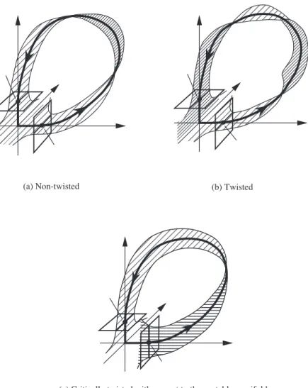
For a generic homoclinic orbit, one can dene its twistedness. Namely in our context, a homoclinic orbit is said to be twisted resp.non-twisted] if the stable manifold forms a M$obius band resp. a cylinder] in a tubular neighborhood of the homoclinic orbit. The inclination-ip homoclinic orbit is then a degenerate situation in such a way that it lies in transition between twisted and non-twisted homoclinic orbits (Figure 6.1). For a historical note, see the following Remark.

Letv be a g-equivariant vector eld on IR³ satisfying (GL1) and, instead of (GL2,3), we assume that it admits an inclination-ip homoclinic orbit ;⁺to the origin O. The symmetry then implies that there exists another inclination-ip homoclinic orbit ;^; =g(;⁺). We call such a pair ; aninclination-ip double homoclinic loop. The following remarkable theorem is due to Rychlik 1990].

Theorem 6.2.

(Rychlik)Letv be ag-equivariant vector eld with an inclination- ip double homoclinic loop to a hyperbolic equilibrium point whose eigenvalues ^ss < ^s<0< ^u satisfy

12 <^;s

^u <1<^;ss

^u (6:1)

and let v be its generic unfolding with v⁰ =v. Then there exists an arbitrarily small such that v possesses a geometric Lorenz attractor.

Here we can take as a two-dimensional parameter.

Remark 6.3. The inclination-ip homoclinic orbit was, to the authors' knowl- edge, rst introduced by Yanagida 1987] for the study of homoclinic doubling bifurcations, although he did not use the terminology \inclination-ip" sug- gested by B. Deng later. In fact Yanagida introduced three types of codimension two degenerate homoclinic orbits which are now called

1. a homoclinic orbit with resonance 11

(a) Non-twisted (b) Twisted

(c) Critically twisted with respect to the unstable manifold

Figure 6.1: An inclination-ip homoclinic orbit.

12

2. an inclination-ip homoclinic orbit 3. an orbit-ip homoclinic orbit,

each of which undergoes a homoclinic doubling bifurcation (Chow-Deng-Fiedler 1990], Kisaka-Kokubu-Oka 1993], Sandstede 1993]). Such homoclinic doubling bifurcations turn out to be closely related to a homoclinic bifurcation giving rise to geometric Lorenz attractors. Indeed, the above theorem due to Rych- lik shows the creation of geometric Lorenz attractors from an inclination-ip double homoclinic loop, and, following Rychlik's work, Robinson proved the birth of geometric Lorenz attractors from a double homoclinic loop with reso- nance (Robinson 1989, 1992]). More recently, it is shown an analogous result for an orbit-ip double homoclinic loop (Kokubu and Oka]), which completes the similarity of homoclinic doubling bifurcations and homoclinic bifurcations generating geometric Lorenz attractors. In this paper we use the Rychlik's the- orem because it is easier to construct an inclination-ip homoclinic loop in an unfolding of a degenerate singularity. See also Oka 1994].

The following is the fundamental observation given by Rychlik 1990]: The equation (5.3) admits a symmetric pair of inclination-ip homoclinic orbits.

Indeed, the rst two equations are independent on the z-variable and are inte- grable due to the Hamiltonian structure. Thus we can obtain the explicit double homoclinic solution (x(t)y(t)) to the hyperbolic equilibrium point (00) where the linearization has the eigenvalues^p. Then we substitute the known func- tion x(t) into the third equation of (5.3) and solve it using the variation of constants formula yielding

z(t) =e^tz(0) +^{Z t}

0

e^;sx(s)²ds: Take z(0) = ^{;Z ;1}

0

e^;sx(s)²ds, namely, we take z(t) =e^{tZ t}

;1

e^;sx(s)²ds: (6:2) We claim that this solution h(t) = (x(t)y(t)z(t)) is an inclination-ip homo- clinic orbit to the equilibrium pointO= (000). In fact, since the eigenvalues at Ois given by^u =^ps=^ss =^;p from the assumption 0<^; <^p, the condition (Ev) is satised. Then the orbit h(t) is indeed homoclinic to O, since x(t) has the following asymptotic behavior:

jx(t)^j=O(e^pt) ast^!;1 and ^jx(t)^j=O(e^;pt) ast^!+¹ 13

from which it is easy to show that z(t)^!0 as t^!1. The same estimate in fact shows that ^jz(t)^j =O(e^t) ast ^!+¹, which veries the condition (Asy).

Finally in order to check the inclination-ip condition, it su!ces to see that the surface given by the direct product of the homoclinic orbit (x(t)y(t)) in the (xy)-plane with the z-axis is invariant under the ow. This implies that the surface is nothing but the stable manifold and at the same time the extended unstable manifold. However, the system (5.3) does not satisfy the condition (6.1) in the Rychlik's theorem, since ^u = ^jssj = ^p, and hence we cannot directly apply the theorem to (5.3). Therefore we need to add more parameters to perturb the equation so that it recovers the desired eigenvalue condition ^u <^jssj without breaking the inclination-ip double homoclinic loop. In the next section we derive a persistence condition for inclination-ip homoclinic orbits, which plays an essential role in our perturbation argument.

7 Persistence of inclination-ip homoclinic orbits

Let _

x

=v(

x

) be ak-parameter family (k 3) of vector elds on IR³ such that, for = 0, the vector eld _

x

= v(

x

0) possesses an inclination-ip homoclinic orbit h(t) to a hyperbolic equilibrium point O. Namely the extended unstable manifoldW^eu(O) is tangent to the stable manifoldW^s(O) along the homoclinic orbit h(t). Let ^sssu be corresponding eigenvalues at O. In this section, we shall study the condition for the persistence of the inclination-ip homoclinic orbit under the perturbation by .

Consider the variational equation alongh(t) for = 0:

u_ =Dv(h(t)0)u

and take the three linearly independent solutionsq⁰(t) = _h(t)q¹(t)q²(t) to the variational equations satisfying the following asymptotic behavior:

jq⁰(t)^j =O(e^ut) ast^!;1 and ^jq⁰(t)^j =O(e^st) as t^!+¹

jq¹(t)^j =O(e^st) as t^!;1 and ^jq¹(t)^j =O(e^sst) as t^!+¹

jq²(t)^j =O(e^sst) as t^!;1 and ^jq²(t)^j =O(e^ut) as t^!+¹: For the proof of the existence of such solutions, see Gruendler 1985] and Kokubu 1988]. Note that these fundamental solutions span tangent spaces of the invariant manifolds along the inclination-ip homoclinic orbit as follows:

T^h(t)W^s(O) =T^h(t)W^eu(O) = span^fq⁰(t)q¹(t)^g T^h(t)W^u(O) = span^fq⁰(t)^g: We regard these solutions as column vector functions and dene the funda- mental matrix solution to the variational equation by

14

V(t) = (q⁰(t)q¹(t)q²(t)): Also we take the projection matrix

P =

0

B

@

0 0 0 0 1 0 0 0 1

1

C

A

and dene the column vector function X(t) =V(t)

"

P ^{Z t}

;1

V(s)^;1@v

@⁽h(s)0)ds+ (I^;P)^{Z t}

0

V(s)^;1@v

@⁽h(s)0)ds

#

:

Theorem 7.1.

The inclination-ip homoclinic orbit persists along a codimen- sion two submanifold ^B in the -space, provided the following two vectors are linearly independent:

M¹ = ^{Z 1}

;1

^b(t)^@@v(h(t)0)dt M² = ^{Z 1}

;1

^b(t)ⁿD²v(h(t)0)X(t) + ^@@ Dv(h(t)0)^oq¹(t)dt

where ^b(t) is a unique (up to constant multiple) bounded solution to the adjoint variational equation

_^

u=^;u^Dv(h(t)0) along the homoclinic orbit h(t).

Furthermore the submanifold^B is perpendicular to M¹ and M² at = 0. Sometimes, it is more convenient to take advantage of special form of equa- tions, namely, the following Corollary holds:

Corollary 7.2.

Suppose the unperturbed system

x

_ =v(

x

0) at = 0 takes the

form x_ = v¹(xy)

y_ = v²(xy) z_ = z+v³(xy)

where the ( _xy_)-equation is a Hamiltonian equation with a homoclinic orbit to a hyperbolic saddle point, say O, and < 0 is a weaker stable eigenvalue at O so that the corresponding homoclinic orbit in the entire vector eld becomes an inclination-ip one. Then the second integral M² for the persistence of the inclination-ip homoclinic orbit is simpli ed to

15

M² =^{Z 1}

;1

^b(t) @

@Dv⁽h(t)0)e(t)dt where e(t) = (00e^t)^T and ^b(t) = ( _y(t)^;x_(t)0).

Proof of Theorem 7.1. The proof mainly follows the idea of Theorem A in Kokubu 1988]. Indeed the derivation of the integral M¹ has been done there, however we give an outline of it here since it is used for the derivation of the other integral M².

Take the inverse of the fundamental matrix V(t) = (q⁰(t)q¹(t)q²(t))

then it gives a fundamental matrix for the adjoint variational equation _^

u=^;u^Dv(h(t)0) (7:1) where ^ustands for a three-dimensional row vector. Let the row vector functions q^ⁱ(t) (i = 012) be dened by

V(t)^;1 =

0

B

@

q^⁰(t) q^¹(t) q^²(t)

1

C

A

which are fundamental solutions to (7.1). In particular, the solution ^q²(t) is a unique (up to constant multiple) non-trivial bounded solution.

The main idea of the proof of Theorem 7.1 is to take a cross section

& = span^fq¹(t)q²(t)^g

transverse to the homoclinic orbit h(t) and to draw perturbed invariant man- ifolds W^u(O )W^s(O )W^eu(O ) on this section &. For this purpose, it is convenient to make the change of variable

x=h(t) +z and to rewrite the original equation as

z_ =Dv(h(t)0)z+N(tz) (7:2) where

N(tz) =v(h(t) +z)^;v(h(t)0)^;Dv(h(t)0)z: (7:3) Furthermore, take the initial condition of z as

16

z(0) = ¹q¹(0) +²q²(0) (7:4) and denote the solution with such an initial condition by

z(t ) = (¹²):

If there is no confusion, we sometimes identify the initial point z(0 ) with itself. Since V(t) is a fundamental matrix, the variation of constants formula convert the equation (7.2) to the following equivalent integral equation:

z(t) =V(t)V(0)^;1z(0) +^{Z t}

0

V(s)^;1N(sz(s))ds: (7:5) The next lemma immediately follows from the denition of the fundamental matrixV(t) and the asymptotic behavior of the fundamental solutionsqⁱ(t) (i= 012).

Lemma 7.3.

(exponential dichotomy) (i) Let P^; be the projection matrix given by

P^; = diag(011) then there exists positive constants K such that

jV(t)(I ^;P^;)V(s)^;1j Ke^;(s;t) (t s0)

jV(t)P^;V(s)^;1j Ke^;(t;s) (s t0) (ii) Let P⁺ be the projection matrix given by

P⁺ = diag(110) then there exists positive constants K such that

jV(t)P⁺V(s)^;1j Ke^;(t;s) (0s t)

jV(t)(I ^;P⁺)V(s)^;1j Ke^;(s;t) (0t s):

Note thatI^;P^; is the projection to T^h(0)W^u(O) andP⁺ is the projection toT^h(0)W^s(O).

Fort0, we decompose (7.5) into

z(t) = V(t)(I ^;P^;)V(0)^;1z(0) +^{Z t}

0

V(s)^;1N(sz(s))ds +V(t)P^;V(0)^;1z(0) +^{Z t}

0

V(s)^;1N(sz(s))ds: 17

From the estimate in the previous lemma, we can show that the rst term of the integral equation stays bounded as t^!;1 whereas the second term diverges to¹ unless

P^;V(0)^;1z(0) +^{Z ;1}

0

V(s)^;1N(sz(s))ds= 0: (7:6) Denote the left hand side by E^;(), then the above condition shows in fact thatE^;() = 0 if and only if ²W^u(O ). By the implicit function theorem, we can solve the equation E^;() = 0 as:

=^;() = (^1;()^2;())

which gives a point of intersection in & with the unstable manifold W^u(O ).

Similarly fort 0, we obtain the condition of the stable manifoldW^s(O ) as:

E⁺() = (I^;P⁺)V(0)^;1z(0) +^{Z 1}

0

V(s)^;1N(sz(s))ds= 0 which has a solution of the form:

² =²⁺(¹)

corresponding to the intersection curve of the stable manifold W^s(O ) with the section &.

Now the set of persistence for a homoclinic orbit is given by

H=^{fj 2;}()^;2+(^;1()) = 0^g and its gradient vector at = 0 is indeed

M¹ =^{Z 1}

;1

^b(t)@v

@⁽h(t)0)dt:

This proves the rst half of Theorem 7.1. For more detail, see Kokubu 1988].

For the persistence of the inclination-ip condition, let us rst take functions given by

h(t) =h(t) +z(t ()) where ^;() = (^1;()^2;())

⁺() = (^1;()²⁺(^;1 ())):

These functions h(t ) converge to the equilibrium point exponentially as t^!1, respectively, since h^;(0 )²W^u(O ) and h⁺(0 )²W^s(O ).

18

Consider the variational equation along these half orbits:

u_ = Dv(h(t ))u

= ^fDv(h(t)0) +R(t)^gu ⁽⁷:7) where

R(t) =Dv(h(t ))^;Dv(h(t)0): Taking the initial condition

u(0) =¹q¹(0) +²q²(0)

we denote the solution to (7.7) by u(t ). Then the similar argument as before yields that = (¹²)²T^h+(0)W^s(O ) if and only if

(I^;P⁺)V(0)^;1u⁺(0 ) +^{Z +1}

0

V(s)^;1R⁺(s)u⁺(s )ds= 0: Since u⁺(s ) is linear in, the latter condition takes the form

K⁺()¹ + (1 +L⁺())² = 0: (7:8) On the other hand, for T^h;(0)W^eu(O ), it is more convenient to consider

w^;(t ) =e^;tu^;(t )

where is a real number satisfying ^ss < < ^s < 0. Clearly ² T^h;(0)W^eu(O ) if and only if w^;(t ) ^! 0 as t ^{! ;1}, or equivalently

jw^;(t )^j remains bounded as t^!;1.

The equation (7.7) with minus-sign then takes w_^;(t) = ^;e^;tu^;(t) +e^;tu_^;(t)

= ^;w^;(t) +^fDv(h(t)0) +R^;(t)^gw^;(t)

= ^f(Dv(h(t)0)^;I) +R^;(t)^gw^;(t) which has a fundamental matrix

W(t) =e^;tV(t)

when= 0, sinceR(t0) = 0. In particular, we have the following exponential dichotomy estimate:

jW(t)(I^;Q^;)W(s)^;1j Ke^;(s;t) (ts0)

jW(t)Q^;W(s)^;1j Ke^;(t;s) (st0) 19

for someK >0, where Q^;= diag(001), that is I^;Q^; is the projection to T^h;(0)W^eu(O ) which is spanned by q⁰(0) and q¹(0).

Now the same argument works for this case as well and we see that = (¹²)²T^h;(0)W^eu(O ) if and only if

Q^;W(0)^;1w^;(0 )^{;Z 0}

;1

W(s)^;1R^;(s)w^;(s )ds

=Q^;V(0)^;1u^;(0 )^{;Z 0}

;1

V(s)^;1R^;(s)u^;(s )ds = 0: From the linearity of u^;(s ) with respect to , the last condition takes the form K^;()¹ + (1 +L^;())² = 0: (7:9) Note that Q^;=I^;P⁺.

The condition for the inclination-ip is therefore given by the equation

;

K^;()

1 +L^;() =^; K⁺()

1 +L⁺() (7:10)

which denes a set ^T in the parameter space. Then the set

C =^H\T

gives the desired set of parameters for which the original equation _

x

=v(

x

) has an inclination-ip homoclinic orbit. Our remaining task is to show that the set ^T denes a local submanifold of codimension one whose gradient vector at = 0 is spanned by the integralsM¹ andM². Then the conclusion of Theorem 7.1 immediately follows from the implicit function theorem.

From the dening equation (7.10) of^T, its gradient vector at= 0 is given by

;(K^;)⁰(0) + (K⁺)⁰(0):

We shall compute the derivatives (K)⁰(0) as follows: First we have

@@

=0

Q^;V(0)^;1u^;(0 )^{;Z 0}

;1

V(s)^;1R^;(s)u^;(s )ds

=^;Q^{;Z 0}

;1

V(s)^;1@R^;

@ ⁽s0)u^;(s 0)ds

;Q^{;Z 0}

;1

V(s)^;1R^;(s0)@u^;

@ ⁽s 0)ds:

Then from the denition of the initial condition u^;(0 ) =¹q¹(0) +²q²(0)

20

and from

R^;(s0) 0

@R^;

@ ⁽s0) = D²v(h(s)0)@h^;

@ ⁽s0) + @

@Dv⁽h(s)0) we have

(K^;)⁰(0) =^{Z 0}

;1

q^²(s)

(

D²v(h(s)0)@h^;

@ ⁽s0) + @

@Dv⁽h(s)0)

)

q¹(s)ds:

Similarly, we have (K⁺)⁰(0) =^{;Z +1}

0

q^²(s)

(

D²v(h(s)0)@h⁺

@ ⁽s0) + @

@Dv⁽h(s)0)

)

q¹(s)ds:

Lemma 7.4.

(i) The function ^@h@;(t0) coincides with the column vector function X(t), namely,

@h^;

@ ⁽t0)

=V(t)

"

P^{Z t}

;1

V(s)^;1@v

@⁽h(s)0)ds+ (I^;P)^{Z t}

0

V(s)^;1@v

@⁽h(s)0)ds

#

: where P =P^;.

(ii) @h⁺

@ ⁽t0)^; @h^;

@ ⁽t0) =V(t)

0

B

@

00 M¹

1

C

A:

From this Lemma, the conclusion of Theorem 7.1 immediately follows, since

;(K^;)⁰(0) + (K⁺)⁰(0) =^;M²+ (const.)M¹: Below we shall prove Lemma 7.4.

Proof. Recall that the function h(t) satises dthd ⁽t) =v(h(t))

and hence ^{dtd @h@}(t0) satises the linear inhomogeneous equation 21

dtd @h

@ ⁽t0) =Dv(h(t)0)@h

@ ⁽t0) + @v

@⁽h(t)0): Therefore we have

@h

@ ⁽t0) =V(t)

(

V(0)^;1@h

@ ⁽⁰0) +^{Z t}

0

V(s)^;1@v

@⁽h(t)0)

)

(7:11) which yields

@h⁺

@ ⁽t0)^; @h^;

@ ⁽t0) =V(t)V(0)^;1 @h⁺

@ ⁽⁰0)^; @h^;

@ ⁽⁰0)

!

=V(t)

0

B

@

00 M¹

1

C

A

from the denition of h(t). This proves the statement (ii).

We shall show the statement (i). Since ^@h@;(t0) converges to 0 ast^!;1, the same argument for obtaining (7.6) applied to (7.11) yields

P

(

V(0)^;1@h^;

@ ⁽⁰0) +^{Z ;1}

0

V(s)^;1@v

@⁽h(s)0)ds

)

= 0: Here we have used that

V(0)^;1@h^;

@ ⁽⁰0) =

0

B

@

^1;00(0) ^2;0(0)

1

C

A=PV(0)^;1@h^;

@ ⁽⁰0):

From this together with (7.11), we obtain the desired equality. This completes the proof of Lemma 7.4 and hence of Theorem 7.1. ²

Now we proceed to the proof of Corollary 7.2.

Proof of Corollary 7.2. The special form of the equation implies that we can choose

q¹(t) = _h(t) +ce(t) where cis a constant.

Lemma 7.5.

q^²(t)

(

D²v(h(t)0)@h

@ ⁽t0) + @

@Dv⁽h(t)0)

)h_(t)

= d dt

(

q^²(t) d

dt @h

@ ⁽t0)

!)

: 22

Proof. Straightforward computation using

dtd q^{^2}(t) =^;q^²(t)Dv(h(t)0)

and d

dt@h

@ ⁽t0) =Dv(h(t)0)@h

@ ⁽t0) + @v

@⁽h(t)0)

prove the desired equality. ²

From this lemma with q¹(t) = _h(t) +ce(t), we have

Z

+1

0

q^²(s)

(

D²v(h(s)0)@h⁺

@ ⁽s0) + @

@Dv⁽h(s)0)

)

q¹(s)ds

=^{Z +1}

0

dtd

(

q^²(t) d

dt @h⁺

@ ⁽t0)

!)

dt +c^{Z +1}

0

q^²(s)

(

D²v(h(s)0)@h⁺

@ ⁽s0) + @

@Dv⁽h(s)0)

)

e(t)ds:

(7:12)

The rst term can be written as

Z

+1

0

dtd

(

q^²(t) d

dt @h⁺

@ ⁽t0)

! )

dt

=

"

q^²(t) d

dt @h⁺

@ ⁽t0)

!#

+1

0

= limt!+1q^²(t) d

dt @h⁺

@ ⁽t0)

!

;q^²(0) d

dt @h⁺

@ ⁽⁰0)

!

=^;q^²(0) d

dt @h⁺

@ ⁽⁰0)

!

since, as t^!+¹, ^q²(t) and ^{dtd @h@+}(t0) both converge to 0 exponentially.

From the special form of the vector eld, we have D²v(h(t)0)e(t) 0 and hence, for the second term of (7.12),

Z

+1

0

q^²(t)

(

D²v(h(t)0)@h⁺

@ ⁽t0) + @

@Dv⁽h(t)0)

)

e(t)dt

=^{Z +1}

0

q^²(t) @

@Dv⁽h(t)0)e(t)dt:

Thus we have obtained

23

(K⁺)⁰(0) = ^;c^{Z +1}

0

q^²(t) @

@Dv⁽h(t)0)e(t)dt +^q²(0) d

dt @h⁺

@ ⁽⁰0)

!

: Similarly, we have

(K^;)⁰(0) =c^{Z 0}

;1

q^²(t) @

@Dv⁽h(t)0)e(t)dt +^q²(0) d

dt @h^;

@ ⁽⁰0)

!

: Therefore the gradient vector to the set ^T at= 0 is given by

;(K^;)⁰(0) + (K⁺)⁰(0) =^;c^{Z +1}

;1

q^²(t) @

@Dv⁽h(t)0)e(t)dt +^q²(0)

(d

dt @h⁺

@ ⁽⁰0)

!

;

dtd @h^;

@ ⁽⁰0)

!)

the rst term of which is nothing but the desired simplied form of M², since, for the special form of vector eld, it is easy to see that bounded fundamental solution ^q²(t) is given by

q^²(t) = ^b(t) = (_y(t)^;x_(t)0): Finally we compute

q^²(0)

(d

dt @h⁺

@ ⁽⁰0)

!

;

dtd @h^;

@ ⁽⁰0)

!)

:

From d

dt@h

@ ⁽t0) =Dv(h(t)0)@h

@ ⁽t0) + @v

@⁽h(t)0) we have

dtd @h⁺

@ ⁽⁰0)^; d dt@h^;

@ ⁽⁰0) =Dv(h(0)0)V(0)

0

B

@

00 M¹

1

C

A and hence

q^²(0)

(d

dt @h⁺

@ ⁽⁰0)

!

;

dtd @h^;

@ ⁽⁰0)

!)

= (const.)M¹:

This completes the proof of Corollary 7.2. ²

24

8 Computation of the integrals

Take the vector eld:

x_ = y

y_ = x^;x³+Ay+Bxz+Cyz z_ = z+x²

where = (ABC) as a perturbation of (5.3) which has an inclination-ip homoclinic orbit.

It is not hard to give all the necessary information explicitly for the computation of the integrals M¹ and M² using the original formula in The- orem 7.1 for this case. Indeed, since the homoclinic solution h(t) is given, it is easy to obtain q⁰(t) = _h(t). The solution q¹(t) is given of the form q¹(t) =q⁰(t) +ce(t) where e(t) = (00e^t)^T and the constantcis chosen so as to satisfy ^jq¹(t)^j = O(e^st) as t ^{! ;1}. For q²(t), we rst consider the Hamil- tonian function H(xy) = ^{y22 ;x22} +^x44 for the (_xy_)-equation with = 0, and note that the homoclinic orbit h(t) corresponds to the energy level H = 0. For any ^;22 < h <0, the energy level curve H(xy) = h gives a periodic solution p(t h). Dierentiate it byh and puth = 0, then we have a solution ^@h@ p(t 0) to the variational equation along the homoclinic orbit for the (_xy_)-equation. For the _z-equation, again we can use the variation of constants formula and hence we obtain the desired solution q²(t). The unique bounded solution ^b(t) to the adjoint equation is simply given as ^b(t) = ( _y(t)^;x_(t)0).

Therefore we can carry out the computation of M¹ and M² using these data. However, it is more convenient to take advantage of the special form of the equation and apply the simplied integrals given in Corollary 7.2.

Now the computation becomes much easier. In fact, M¹ =^{Z 1}

;1

( _y(t)^;x_(t)0)

0

B

@

0 0 0

y(t) x(t)z(t) y(t)z(t)

0 0 0

1

C

Adt

=^{Z 1}

;1

(^;x_(t)y(t)^;x_(t)x(t)z(t)^;x_(t)y(t)z(t))dt M² =^{Z 1}

;1

( _y(t)^;x_(t)0)

0

B

@

0 0 0 0 0 0 0 0 0

0 1 0 z(t) 0 x(t) 0 z(t) y(t)

0 0 0 0 0 0 0 0 0

1

C

A 0

B

@

00 e^t

1

C

Adt

=^{Z 1}

;1

(0^;x_(t)x(t)e^t;x_(t)y(t)e^t)dt:

25