Title A spatial-temporal random process for geotechnical design basedon observation method( 本文(Fulltext) )
Author(s) RUNGBANAPHAN PONGWIT
Report No.(Doctoral Degree) 博士(工学) 甲第383号 Issue Date 2010-03-25 Type 博士論文 Version publisher URL http://hdl.handle.net/20.500.12099/33544 ※この資料の著作権は、各資料の著者・学協会・出版社等に帰属します。
A spatial-temporal random process for geotechnical
design based on observational method
時間―空間確率過程を用いた観測法に基づく地盤設計法
by
Pongwit Rungbanaphan
Gifu University, Japan
February 2010
A spatial-temporal random process for geotechnical design
based on observational method
時間―空間確率過程を用いた観測法に基づく地盤設計法
A dissertation submitted in partial fulfillment of the requirements for the doctoral degree in engineering
by
Pongwit Rungbanaphan (1073812105)
under the supervision of Prof. Yusuke Honjo
Examination Committee: Prof. Nobuoto Nojima (chair)
Prof. Yusuke Honjo Prof. Atsushi Yashima Prof. Ikumasa Yoshida
Department of Civil Engineering Gifu University
Japan February 2010
Abstract
This research proposes a methodology for geotechnical design based on spatial-temporal random process using the observational method. Temporal soil behavior is introduced based on geotechnical models which describe ground behavior at an arbitrary point with time through the unknown parameters employed in the model, while the spatial correlation of the soil behaviors is introduced through the spatial correlation of these unknown parameters. The method is based on Bayesian estimation by considering both prior information of the unknown parameters, including spatial correlation, and observation data of the ground behavior to search for the best estimates of the parameters at any arbitrary points on the ground. The optimized selection of auto-correlation distance and observation error by Akaike’s Bayesian Information Criterion (ABIC) is also proposed. It is proved in this study that, for the static problem without process noise, the Kalman filter yields identical results with those from the Bayesian estimation. The use of Kalman filter formulation to introduce process noise into the proposed spatial-temporal process is described. The ordinary kriging technique is presented as an alternative approach for spatial interpolation of the unknown parameters, which in fact is included in the proposed formulation in the form of simple kriging, and the difference between the approaches is also discussed.
The application in prediction of primary consolidation by Asaoka’s method and secondary compression settlement by S ~ log(t) method is presented as the application examples of the proposed method. Several case studies were carried out using both simulated settlement data and actual field observation data to investigate the performance of the proposed approach. It is concluded that the accuracy of the settlement prediction can be improved by taking into account the spatial
correlation structure and the proposed approach gives the rational prediction of the settlement at any location at any time with quantified uncertainty. The sensitivity of this improvement to variations in the auto-correlation distance, observation spacing, and number of observation points is investigated. The accuracy of the estimation of auto-correlation distance, observation error, and the final settlement at an arbitrary location is also discussed. In addition, it was found that, by including process noise in the calculation, one can introduce a kind of forgetting factor which actually gives more weight to the more recent observation and improve prediction. However, care should be taken in choosing this forgetting factor in order to optimize the prediction.
Acknowledgement
First and foremost, I would like to express my sincere gratitude to my advisor, Prof. Yusuke Honjo, not only for his enthusiastic guidance and continuous support throughout my research, but also his kind encouragement and supports during the program.
I am deeply indebted to Prof. Ikumasa Yoshida from the Tokyo City University. His valuable suggestions and comments helped me in all the time of research.
Furthermore, I would like to thank the members of my thesis committee, Prof. Nobuoto Nojima and Prof. Atsushi Yashima for spending their precious time reading my thesis and making valuable suggestions.
I heartily appreciate Monbukagakusho for generous financial support. Without its support, my ambition of doctoral study can hardly be realized.
My warm thanks are also due to my buddies and all my lab friends for their kind help and encouragement in my study and life in Gifu.
Finally, I would like to give my special thanks to my beloved family members for their love, encouragement, and care all along the road to pursue my educational goals.
Table of contents
Abstract ………..…….…i
Acknowledgement ……..………..….iii
Table of contents………..………..iv
List of tables………..………vii
List of figures ………....…..viii
Notations ………...xii
1. Introduction ………..1
1.1 Background ………..………1
1.2 Objective and scope ……….…3
1.3 Organization of the dissertation ………...5
2. Literature review ………..………...8
2.1 Uncertainties in geotechnical engineering ……..……….8
2.1.1 Introduction ………..8
2.1.2 A proposed view for uncertainty classification ……….11
2.1.3 Dealing with uncertainty ………13
2.2 The observational method for reliability analysis ………..14
2.2.1 The observational method in geotechnical design ……….14
2.2.2 Settlement prediction by the observational method ………..…15
2.3 Spatial-temporal modeling of soil behavior ………..………18
2.3.1 Spatial and temporal variability of soil behavior ………..18
2.3.2 Modeling the spatial variation………19
2.3.3 Modeling the temporal variation ………23
2.3.4 Spatial-temporal model ……….24
3. Spatial-temporal process ……….………..29
3.1 Basic assumptions ………..29
3.1.1 Major assumptions ……….29
3.1.2 Minor assumptions ……….30
3.2 Bayesian estimation considering spatial correlation structure ………...31
3.2.1 Observation model ……….31
3.2.2 Prior information model ………32
3.2.3 Bayesian estimation………35
3.3 Model selection: Akaike’s Bayesian Information Criterion ……….……….36
3.4 Process noise consideration by the Kalman filter method ……….…………38
3.5 Local estimation by the kriging method ………40
4. Application examples ……….………43
4.1 Primary consolidation settlement prediction by Asaoka’s method………43
4.1.1 Settlement prediction model ………..43
4.1.2 Simulation experiment ……….…………..45
4.1.2.1 Random field generation by frequency-domain technique ………….………….45
4.1.2.2 Improvement of the estimation by considering spatial correlation structure …..48
4.1.2.4 Estimation of final settlement at an arbitrary location ……….…55
4.2 Secondary compression prediction by S ~ log(t) method ………….……….57
4.2.1 Settlement prediction model ………..57
4.2.2 Simulation experiments ……….59
4.2.2.1 Random field generation by frequency-domain technique ……….59
4.2.2.2 Improvement of the estimation by considering spatial correlation structure …...59
4.2.2.3 Estimation of settlement at an arbitrary location ……….………62
4.2.3 Case study using actual observation data ……….……….63
4.2.3.1 Description of the case ……….………63
4.2.3.2 Estimation of auto-correlation distance and observation error ………65
4.2.3.3 Settlement estimation and prediction ………..……….66
4.2.3.4 Effect of process noise consideration………..……….69
5. Summary and conclusion ………..…95
References ……….……….100
Appendices A. Derivation of Kalman filter formulation based on Bayesian approach ………..……108
B. Derivation of kriging formulation based on Bayesian approach ………112
C. Kriging techniques: assumptions and equations ……….118
D. Derivation of spectral density function ………..…119
E. Field observation data of secondary compression in peat………128
List of tables
4-1 Comparison of estimation error between the cases with considering and ignoring spatial correlation for different n and s/η ratios, using 2-D simulations of 100 times (Nsim = 100) by
Asaoka’s model, assuming σε = 1.0 cm and Tv = 0.164………70
4-2 Estimation error of auto-correlation distance (η) and standard deviation of observation error (σε) for different n, L/η ratios and s/η ratios, using 2-D simulations of 100 times (Nsim = 100)
by Asaoka’s model, assuming σε = 1.0 cm and Tv = 0.164……..………72
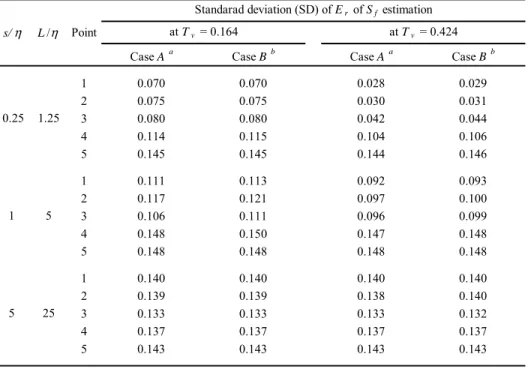
4-3 Estimation error of final settlement at arbitrary points (point 1 to 5 in Fig. 4-9) for different s/η ratios, L/η ratios and Tv, using 2-D simulations of 100 times (Nsim = 100) by Asaoka’s model,
List of figures
1-1 A scheme of the proposed spatial-temporal estimation method ………..………..…7 2-1 Uncertainties in geotechnical design ……….………..…27 2-2 An example of subsoil investigations at two different sites ………..………..…27 2-3 Conceptual models of spatial-temporal process when are viewed as (a) a set of random
functions (RF) Zi(x), i = 1, 2, . . . T ; and (b) a set of vectors of time series (TS) Zα(t), α = 1,
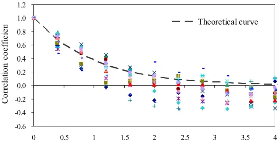
2, . . . n (Kyriakidis and Journel 1999)………...…28 4-1 Correlation coefficient-distance relationship of the generated random values, comparing with
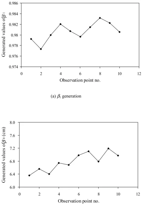
the theoretical curve, for 1-D simulation ……….…73 4-2 Examples of the generated values of Asaoka’s model parameters (β1, β0) for 1-D simulation,
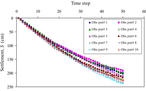
assuming n = 10 and s/η = 0.2 ……….…74 4-3 Examples of the generated settlement with time for 1-D simulation by Asaoka’s model,
assuming n = 10, s/η = 0.2 and σε = 1.0 cm ………75
4-4 Stepwise updating for estimation of the model parameters (β1, β0) for 1-D simulation by Asaoka’s model, assuming n = 10, s/η = 0.2 and σε = 1.0 cm ………76
4-5 Comparison of estimation error between the cases with considering and ignoring spatial correlation at each observation point at 50th time step for 1-D simulation of 1000 times (Nsim =
1000) by Asaoka’s model, assuming n = 10, s/η = 0.2 and σε = 1.0 cm ……….77
4-7 Stepwise updating for estimation of the model parameters (β1, β0) and final settlement at point A (see Fig. 4-6) for 2-D simulation by Asaoka’s model, assuming n = 36, s/η = 0.5 and σε =
1.0 cm ………..………79
4-8 Estimation error vs. time factors for 2-D simulation of 100 times (Nsim = 100) by Asaoka’s model, assuming n = 36, s/η = 0.5 and σε = 1.0 cm ………80
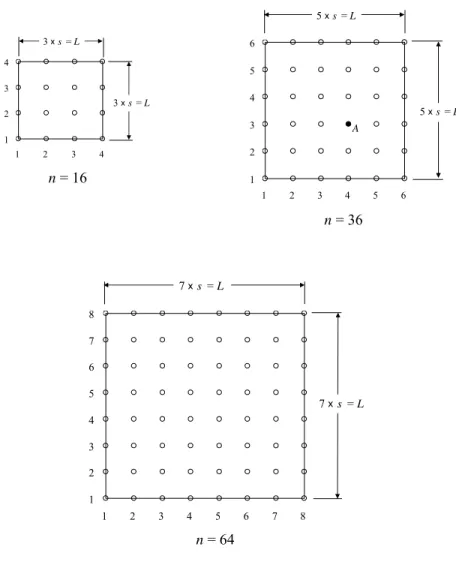
4-9 Observation plan and locations of arbitrary points to be estimated ………….………81
4-10 Estimation error vs. observation time for 2-D simulation of 50 times (Nsim = 50) by S ~ log(t) model, performing at the observation points, assuming n = 36, s/η = 0.25 and σε = 10 cm ………..……82
4-11 Estimation error vs. s/η ratios for 2-D simulation of 50 times (Nsim = 50) by S ~ log(t) model, performing at the observation points based on the data from the day 10th to 100th, assuming n = 36 and σε = 10 cm ………….………..………83
4-12 Estimation error vs. observation time for 2-D simulation of 50 times (Nsim = 50) by S ~ log(t) model, performing at the removed observation points, assuming n = 36, s/η = 0.25 and σε = 10 cm ………....……….………84
4-13 Estimation error vs. s/η ratios for 2-D simulation of 50 times (Nsim = 50) by S ~ log(t) model, performing at the removed observation points based on the data from the day 10th to 100th, assuming n = 36 and σε = 10 cm ………….………85
4-14 Soil condition of a land development site, selected as a case study for settlement prediction based on actual observation data ……….………86
4-15 Surcharge thickness and settlement versus time ……….…….………86
4-16 Location plan of the observation points and surcharge area ………...……….………87
4-18 Observed settlement versus time (after surcharge removal) with trend line for the data observed at point A in Figure 4-16 ………..………88 4-19 An example of contour of ABIC for estimation of auto-correlation distance (η) and the
standard deviation of the observation error (σε), using observation data until the last step of
observation (the day 1017th)……….………88 4-20 Plots of estimated values of auto-correlation distance (η) and the standard deviation of the
observation error (σε) vs. observation times, for the estimation based on the actual observation data of secondary compression……….………89 4-21 Estimation error vs. observation time for estimation of secondary compression at the last step
of observation (the day 1017th) at the observation points by S ~ log(t) method, using actual observation data ………..……….………90 4-22 Comparison between the estimated settlement and the observed settlement for secondary
compression estimation by S ~ log(t) method based on the actual observation data from the day 103rd to 696th to predict settlement at the day 1017th at the removed observation points ……….……….………91 4-23 Comparison between the estimated settlement, shown as surfaces, and the observed settlement,
shown as points, for secondary compression estimation by S ~ log(t) method based on observed data from the day 103rd to 696th to predict settlement at the day 1017th at the removed observation points ……….………92 4-24 Estimation errors vs. observation times for estimation of secondary compression at the
removed observation points by S ~ log(t) method, using actual observation data ……….……….………93
4-25 Estimation error vs. observation time with different levels of process noises, for estimation of secondary compression at the last step of observation (the day 1017th) at the observation points by S ~ log(t) method, using actual observation data ………….……….………..94 D-1 Auto-correlation function for one-dimensional random process ……….………..…………125 D-2 Spectral density function for one-dimensional random process …..………..125 D-3 Auto-correlation function for two-dimensional random process …..….………126 D-4 Spectral density function for two-dimensional random process …….….………..……127
Notations
a constant parameter, representing the level of process noise c normalizing constant for Bayesian updating formulation
Cij constant coefficient, formulating the trend components for the unknown
parameters zi (i = 1, 2, ... , P; j = 1, 2, ...)
Er error ratio
E[X] mean of random variable X
E[g(X)] mathematical expectation of a given function g of random variable X In,n n × n unit matrix
K total number of observation time step Kk Kalman gain at time step k
k observation time step
k/l subscript, representing the kth step estimation conditioned on processing observation data up to the lth datum
L the total width of the group of observation points
Mk coefficient matrix, relating unknown parameters to observation data at
observation time step k (Yk)
M in,n n × n coefficient matrix, relating unknown parameter zi to observation data Yk
m total number of observation points (n), including unobserved points at which the unknown parameters are to be estimated (m-n)
m0, m1 constant parameters for secondary compression model (S ~ log(t) method) 0
ˆ ( )j
1,0 ˆ ( )j
m x , mˆ ( )0,0 xj prior means of m1 and m0 at point xj
Nsim total number of simulations
n total number of observation points P total number of unknown parameters
Qk covariance matrix of process noise at time step k
S ground settlement S(ω), S(ω1,ω2) spectral density function
Sk settlement vector at kth step of observation
Sk(xj) observed settlement at an observation point xj at observation time step k
Sf final settlement
s spacing of observation points Tv time factor
t time
t0 time at a beginning stage
tf time at a spot of time in the future
tk time at observation time step k
t(x) value of the trend at location x u(x) random component at location x
VC auto-covariance matrix
Vε covariance matrix of observation error VZ covariance matrix of unknown parameter
wij kriging weights attached to the data at each of the observation points
xj spatial vector coordinate at point xj, i.e. (xj’, yj’)
xj’ x coordinate at point xj
x1, x2, … , xn observation points
xn+1, xn+2, … , xm any arbitrary points at which the unknown parameters are to be estimated
Y set of all observation data for the concerned soil behavior Yk observation vector at observation time step k
yj’ y coordinate at point xj
yk(xj) observation data at an observation point xj at observation time step k
Z unknown parameter vector ˆ
Z best estimator of unknown parameter vector for a discrete spatial point field Zoi estimate of the unknown parameter zi at observation points
Zri estimate of the unknown parameter zi at unobserved arbitrary points
Z0 prior mean vector of unknown parameter
zi(x) random function of an unknown parameter zi at an arbitrary point x
ˆ ( )i j
z x estimate of unknown parameter zi at point xj
z0,i(xj) prior mean of unknown parameter zi at point xj
β1, β 0 constant parameters for the Asaoka’s model
1 ˆ ( )xj
β , βˆ ( )0 xj estimates of β1 and β 0 at point xj
) ( ˆ 0 , 1 xj
β , )βˆ0,0(xj prior means of β1 and β0 at point xj
δ vector representing uncertainties of unknown parameters δu scale of fluctuation
η auto-correlation distance μj Lagrange multiplier
ρ(|xi - xj|) auto-correlation function
σ2
m1,0, σ2m0,0 prior variance of m1 and m0
σ2
or variance of interpolation by ordinary kriging
σ2
zi prior variance of the an unknown parameters zi
σ2
β1,0, σ2β0,0 prior variance of β1 and β 0 σε2 variance of the observation error
φjk random phase angles, uniformly and independently distributed in the interval
(0,2π)
ω, ω1, ω2 circular frequency domain 0n,m n × m zero matrix
1 Introduction
1.1 Background
Behavior of geotechnical structure, such as settlement and movement of soil mass, possesses variability in both space and time. The spatial variation of the behavior mainly stems from the natural variability of soil properties. The temporal variation, on the other hand, is due to the complexity of the time-dependent behavior of soil, e.g. consolidation settlement and undrained creep. The influence of these variations can be significant for several design problems in geotechnical engineering practice–for example, the evaluations of differential settlements of structures.
To cope with these variations, a number of approaches have been proposed in several past literatures. For modeling spatial variability, soil property is known to be correlated spatially, for which the property tends to similar in value at closely neighboring points than at widely spaced points (Lumb 1974, Vanmarcke 1977a, DeGroot and Baecher 1993, Baecher and Christian 2003). This naturally induces the spatial correlated characteristic of the resulting soil behavior. By recognizing this fact, the spatial correlation of soil properties has been proposed to be considered in various kinds of geotechnical analysis, such as stability of earth slopes (e.g. Vanmarcke 1977b), foundation settlement (e.g. Fenton and Griffiths 2005), and liquefaction risk (e.g. Fenton and Vanmarcke 1998). As for the temporal variability, the observational method has been considered as an efficient and reliable approach to deal with the uncertainty originated from the time-dependent behavior of soil, by which the design can be calibrated dynamically using the periodically observed data. Since the essence of the method has been emphasized by Peck (1969), the observational
method has been proved to be a practical way to control the uncertainties in designing geotechnical structure, such as excavation (e.g. Young & Ho 1994), tunnel construction (e.g. Iwasaki et al. 1994), and embankment construction (e.g. Wakita and Matsuo 1994). Matsuo and Asaoka (1978) also presented a probabilistic approach for updating the design based on the observation data and named it as dynamic design procedure.
Unfortunately, most of the proposed approaches in past literatures provided only the means to deal with spatial and temporal uncertainties separately. To predict behavior of soil at a particular location and at a spot of time in the future, an approach which incorporates both spatial and temporal variability in the estimation process is needed. The researches in spatial-temporal modeling have been relatively active in such field of study as environmental science, meteorology, hydrology, and reservoir engineering. In geotechnical engineering, however, this research topic has still seldom been concerned. The particular characteristic of the geotechnical problem is that the temporal soil behavior is generally possible to be predicted based on the physical model which directly relates to soil properties. By introducing spatial correlation of soil properties into this temporal model, it is therefore natural to expect that the accuracy of the soil behavior prediction should be improved because, in this case, the data observed from all observation points can be rationally utilized. Furthermore, the rigorously prediction of the ground behavior at any arbitrary points at any time can be possible through this spatial-temporal estimation process. This study is actually an attempt to search for such an approach.
1.2 Objective and scope
The objective of this research is to propose a practical approach which takes into account spatial correlation of soil parameters in the prediction of temporal behavior of geotechnical structure using the observation data. Two main advantages are expected to be achieved:
1. The accuracy of the prediction is improved by systematically utilizing observation data from all observation points.
2. The rigorous prediction at any point and any time can be done with quantified uncertainty.
The proposed approach is established based on the assumption that the soil behaviors are observed at discrete points and discrete time, and this observation data is used to update the unknown parameters employed in the temporal soil model (hereinafter called the ‘unknown parameter’ or ‘model parameters’), by which the soil behavior at a specific time can be predicted through the linear relationship between these unknown parameters and behavior. The spatial correlation structure of the soil behavior is also introduced through these unknown parameters. It should be noted that because the future behavior is to be predicted based on the model parameters which are derived from the observed behavior, the uncertainty of the miscellaneous effects which influence the geotechnical behavior such as external loading uncertainties have already been included in the model.
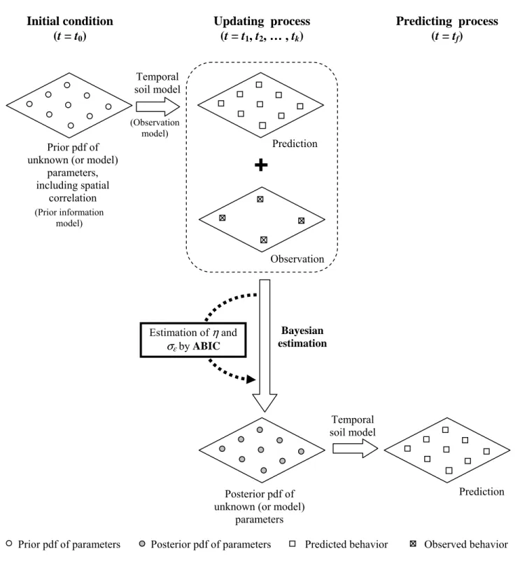
The proposed spatial-temporal estimation method can be illustrated as shown in Figure 1-1. At the beginning stage (t = t0), the statistical parameters of the prior probability distribution function (pdf) of the unknown parameters at discrete points on the ground, including the observation points and the points to be estimated, are required to be input. This can be obtained from the past experience or inferred from the soil testing results. The spatial correlation of the unknown parameters is also introduced in the variation components of prior pdf. Based on this prior pdf, the concerned behavior of soil at each observation time step (t = t1, t2, … , tK) can be predicted through
the selected temporal soil model (also referred as ‘observation model’ in this thesis). Comparing this prediction with the observation data, the statistics of the unknown parameters at each point are updated through the proposed formulation based on the Bayesian estimation. To emphasize, Bayesian approach is chosen to introduce the spatial correlation into the temporal soil model in this research due to its ability to systematically combine the subjective information, i.e. the prior information including the spatial correlation of the unknown parameters, and objective information, i.e. the observation data. Finally, based on these updated estimates of the unknown parameters, the soil behavior at a spot of time in the future (t = tf) can be predicted using the temporal soil model.
Due to the fact that spatial correlation structure is controlled by auto-correlation distance (η), the estimation of this key parameter is necessary. By considering this as a model selection problem, it will be shown that, within the Bayesian framework, auto-correlation distance (η) and the standard deviation of observation error (σε) can be appropriately selected based on Akaike’s Bayesian Information Criterion (Akaike 1980, Honjo and Kashiwagi 1999).
Two well-known techniques are also presented as alternative methods which can replace some parts of the proposed approaches. Firstly, Kalman filter (Kalman 1960, Kalman & Bucy 1961), including spatial correlation of the unknown (or model) parameters, can be use to update the statistics of the parameters based on the observation data. It is proved herein that this process is actually identical to the proposed approach when process noise in the time updating process of Kalman filter is ignored. The effect of process noise consideration is also discussed in this thesis. Secondly, the use of kriging technique (Krige 1966, Matheron 1973) for interpolating values of the unknown parameters to an arbitrary point is also presented. The fact that the interpolation process included in the proposed approach is actually equivalent to the simple kriging technique is
emphasized and the alternative use of ordinary kriging technique for the interpolation is also discussed.
In order to investigate the practical performance of the proposed approach, the applications of the proposed formulation in spatial-temporal prediction of primary consolidation and secondary compression settlement are presented in this thesis. Asaoka’s method (Asaoka 1978), which is an autoregressive model representing a trend equation of time series data of settlement, is chosen as a prediction model for primary consolidation settlement. For the prediction of secondary compression settlement, the S ~ log(t) method (Bjerrum 1967, Garlanger 1972, Mesri et al. 1997), which represents linear relationship between logarithm of time and settlement, is used.
Both simulated data and actual observation data are used as the input for calculations under several test conditions. For the case of simulated data, the settlement data are generated based on the assigned spatial correlation structure of the unknown (or model) parameters using frequency domain technique (Shinozuka 1971, Shinozuka and Jan 1972). Based on this generated settlement data, the statistical inferences of the unknown parameters are back-calculated using the proposed approach. As for the case of actual observation data, the observed settlement of preloaded peat ground site in a suburb area of Tokyo, Japan, is used. This is treated as secondary compression settlement and modeled by S ~ log(t) method. The calculation results of all cases will be presented and discussed in detail later in this thesis.
1.3 Organization of the dissertation
The introductory chapter is followed by Chapter 2 which is devoted to a review of previous literatures associated with this study. Chapter 3 presents the basic assumptions and formulations of the proposed spatial-temporal estimation process. The uses of Kalman filter and kriging technique as the alternative approaches are also discussed in this chapter. Chapter 4 introduces the examples for
practical applications of the proposed approach in geotechnical design and the discussion of the results. The chapter is divided into 2 main sections. Section 4.1 exhibits an example of the primary consolidation settlement prediction by Asaoka’s method using simulated data, while Section 4.2 presents an example of secondary compression prediction by S ~ log(t) method using both simulated and actual observation data. Finally, the summary and conclusion of the research are given in Chapter 6.
Figure 1-1: A scheme of the proposed spatial-temporal estimation method. Initial condition (t = t0) Updating process (t = t1, t2, … , tk) Predicting process (t = tf) Prior pdf of unknown (or model)
parameters, including spatial correlation Prediction Observation Temporal soil model Temporal soil model Posterior pdf of unknown (or model)
parameters Bayesian estimation Prediction Estimation of η and σε by ABIC
Prior pdf of parameters Posterior pdf of parameters Predicted behavior Observed behavior (Observation
model)
(Prior information model)
2 Literature review
2.1 Uncertainties in geotechnical engineering
2.1.1 Introduction
Geotechnical engineers are always dealing with significant level of uncertainties, relating to geotechnical works. Natural soils are known to be heterogeneity, for which the soil properties are different from one spatial location to another inside the soil mass. These variations, basically, cannot be completely investigated. In practice, extensive subsoil investigations are usually constrained by financial possibility. At these selected locations of soil investigations, soil properties are acquired either by field or laboratory tests. These measured properties, which may need to be transformed through empirical or theoretical model to achieve for the design parameters, are then used as the input parameters of geotechnical models or design techniques for predicting pertinent behaviors of the geotechnical structures or evaluating the stabilities of the structures.
Several sources of uncertainties can be clearly observed from the above design process. In addition to the inherent spatial variation of natural soil, the measurement, model, and statistical uncertainties can be expected. Traditional engineering practice tends to adopt a factor of safety in the design in order to cope with these unexpected uncertainties. In 1970, however, Wu and Kraft presented an approach to quantify geotechnical uncertainties and to study the effect of these uncertainties on the reliably of a slope. By this approach, various sources of uncertainty can be systematically compared, analyzed and combined using the probabilistic procedure. Despite these
attractive benefits, however, the geotechnical professions have been somewhat reluctant to use this new method in practice. This might be due to the fact that they have seen little need to adopt the more complex and untried probabilistic method in stead of using the deterministic method which they have plenty of lessons learned from years of professional practice.
However, recent years have shown the trend that the geotechnical uncertainties are required to be treated in the more quantitative way. Geotechnical engineers have been increasingly forced by regulatory agencies or project decision makers to provided quantitative answers about reliability of their design, especially for the large scale or risky structures. Moreover, Load and Resistance Factor Design (LRFD), which are based on reliability methods, are now being introduced into such areas as pile design for highway structure. Due to these facts, the demands for the studies on applications of reliability methods in geotechnical engineering have been increased over the past decades. There has been steady steam of publications on geotechnical engineering in various topics such as environmental geotechnology (e.g. Bogardi et al.1989 and 1990), offshore foundation (e.g. Wu et al.1989, Ronold and Bjerager 1992), effect of geologic anomalies (e.g. Baecher 1979, Tang 1987, Halim and Tang 1993), statistical evaluation of soil properties (e.g. Kulhawy et al.1991, Phoon and Kulhawy 1999a & 1999b), probabilistic slope stability analysis (e.g. Li and Lumb 1987, Chowdhury et al.1987, Honjo and Kuroda 1991, Griffiths and Fenton 2004), and problems related to earthquake hazards (e.g. Fenton and Vanmarcke 1998, Juang et al.2002).
Regardless of the types of problems to be tackled, the most important step for reliability analysis of geotechnical structure is perhaps to define and quantified the components of uncertainties. However, the characterization of geotechnical uncertainties can be a tough task due to the complexity of the sources of uncertainties and even the confusing terminologies. The evidence of these difficulties is the fact that both the classified sources of uncertainties and terms used to explain
them are usually different among the authors. For example, Wu (2009) designated that the uncertainties in geotechnical design are consisted of random and systematic uncertainties. Based on his view, soil variability is the most important source of random error, while inaccuracy or simplifications in material and analytical models are the common sources of systematic errors. It seems that his classification roughly separates inherent variability of soil from the model uncertainties, which include parameter transformation model and analytical model. On the other hands, Baecher and Christian (2003) provided more extensive classification of uncertainties by categorizing into natural variability, knowledge uncertainty, and decision model uncertainty. Natural variability, also referred as aleatory uncertainty, represents the inherent randomness of natural process both spatially and temporally. Knowledge uncertainty, also referred as epistemic uncertainty, is attributed to the lack of information about events and processes which contains site characterization uncertainty, model uncertainty, and parameter uncertainty. Finally, for implementation of the design in practice concerning the economic issues, decision model uncertainty is proposed to be concerned in the calculations.
Focusing on the uncertainties in soil parameter estimates, Tang (1993) classified these uncertainties into three main components, namely inherent variability, statistical uncertainty, and systematic uncertainty which, in this case, is contributed by the inability of a test to reproduce the in situ property due to factors such as sample disturbance, limited specimen size, etc. Phoon and Kulhawy (1999a), however, indicated that three primary sources of uncertainties in soil property estimation consist of inherent variability, measurement error, which is comparable to systematic uncertainty presented by Tang (1993), and transformation uncertainty, which results from the empirical or theoretical model used to relate measure quantities to design parameters.
2.1.2 A proposed view for uncertainty classification
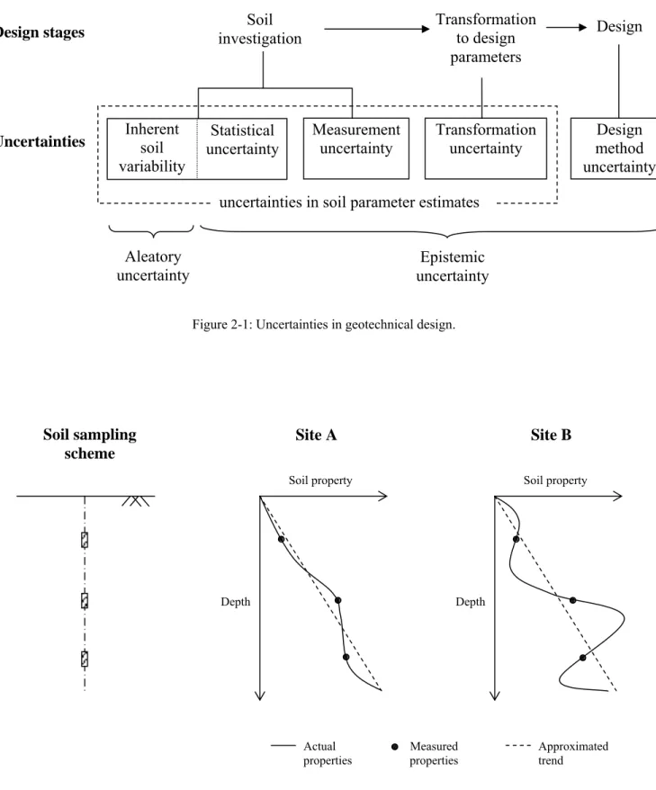
Based on the above review of several past literatures about classification of geotechnical uncertainties, one found inconsistency mainly in terminologies used for defining different sources of uncertainties. In this thesis, an attempt has been made to reorganize categories of geotechnical uncertainties in the more systematic way based on the most commonly used terminology found in the reviewed literatures. This proposed classification is presented in Figure 2-1.
The uncertainties at the different design steps are clearly classified and also grouped to summarize all viewpoints of the uncertainties. During subsoil investigation, the uncertainties consist of (i) combination between inherent soil variability, which primarily results from the natural geologic process, and statistical uncertainty, which is contributed by the statistical assumption or limited number and location of samples, and (ii) measurement uncertainty, which is due to equipment, procedure-operator, and random testing effects. The field or laboratory measurements are then transformed into design soil parameters using empirical or other correlation models. The uncertainty arises at this step is termed transformation uncertainty. Finally, the transformed parameters are put into analytical models or selected design techniques for designing geotechnical structure. Clearly, uncertainty at this step, namely design method uncertainty, arises from the error of using the model to predict the complicated actual soil behavior. It is only the inherent soil variability which is classified as aleatory uncertainty, indicating that this is the only source of uncertainty which cannot be reduced by any observers.
It should be noted that the contribution of the inherent soil variability and statistical uncertainty is freshly proposed in the combined form. This is based on the perspective that these two uncertainties cannot be separated completely, by which one can be induced by another. This
conclusion is illustrated by an example of subsoil investigations at two different sites with the same soil sampling scheme as shown in Figure 2-2.
Figure 2-2 presents an example of subsoil investigations at two different sites, namely site A and site B, showing the measured properties and the approximated trends along with the actual properties. It is assumed that three soil samples are taken at the same depths from both sites and the measured soil properties are also identical at each corresponding depth. No doubt, one must obtain the same linear trend, with depth, of the measured properties at both sites. However, it can be clearly seen from Figure 2-2 that it is only at Site A that the approximated trend can be a good representative of the actual properties. This is because the spatial variation of the properties at site B is much greater than those at site A. It appears that the statistical uncertainty for the current soil investigation at site B is quite significant and the shorter interval of soil samplings is required to acquire for better description of the actual condition, despite the fact that the soil sampling scheme and the trend component are not different from those of site A. This significant amount of statistical uncertainty at site B is induced by the vertical variation of the pertinent soil properties. It should be noted that this conclusion is also applicable for the case of horizontal variation, i.e. when the horizontal trends of soil properties are to be observed. This example illustrates the relation between these two sources of geotechnical uncertainties. Therefore, they are proposed in the combined form as shown in Figure 2-1.
In addition to the inherent spatial variation of soil, the statistical uncertainty also depends on the design situation. This should also be mentioned here in order to provide a comprehensive description of uncertainty in soil property characterization. Honjo and Setiawan (2007) emphasised the essence of classifying the estimations of geotechnical parameters into two different types, namely local estimation and general estimation, in accordance with the corresponding design
situation. Local estimation refers to the situation that the estimation is needed to be performed at a specific spot, e.g. right at the spot where a structure is to be built. General estimation, on the other hand, refers to the case that the estimation is needed to be done generally at any arbitrary location in a certain area, i.e. a reclaimed area where a container yard is to be located. In local estimation, because the location to be design has been predefined, it is possible to reduce the statistical uncertainty by considering relative spatial location between the field exploration point and the concerned structure, e.g. performing kriging technique (Krige 1966, Matheron 1973). In general estimation, however, because targeted estimation value is expected to represent the pertinent soil property of a large area, the statistical uncertainty is inevitably greater than that of the local estimation. Moreover, the difference of the uncertainty levels between these two types of estimation also depends on the spatial correlation condition of the soil property (Honjo and Setiawan 2007). This emphasizes the strong relation between statistical uncertainty and the inherent soil variability.
2.1.3 Dealing with uncertainty
After the uncertainties in geotechnical design have been clearly classified, a problem arises that how one can perform the satisfactory design despite these underlying uncertainties. Wu (2009) states that two principle components of geotechnical design are the (i) calculated risk, i.e. reliability-based design and (ii) the observational method. The reliability-based design involves the evaluation of the failure probability of the structure, whose comprehensive formulation was firstly provided by Freudenthal (1947). The use of first-order second moment (FOSM) method is then introduced as a more convenient approach for evaluation of failure probability (Cornell 1969). An improvement over FOSM is the use of first-order reliability method (FORM) (Hasofer and Lind 1974). More elaborate are stochastic and simulation method (Fenton and Griffiths 2002). The detail explanations
of these techniques for reliability-based design in geotechnical engineering are well documented in Phoon (2008).
The important role of the observational method in solving complex design problems has been recognized since it was proposed by Terzaghi and was detailed described by Peck (1969). Through Bayesian updating, the observational method can also be used to enhance the performance of reliability analysis (Matsuo and Asaoka 1978). This thesis proposes an approach for dealing with spatial-temporal variation of geotechnical problem using the observational method. It should be emphasized here that the proposed approach focuses on providing the local estimation (as mentioned above) by taking into account spatial correlation of geotechnical parameters. Next section presents the review of past literatures in the application of the observational method for reliability analysis.
2.2 The observational method for reliability analysis
2.2.1 The observational method in geotechnical design
Basically, it was seldom technically or economically possible for geotechnical engineer to design for all unfavorable situations. Terzaghi and Peck (1967) states that the significant savings can be made by designing on the basis of the most probable rather than the most unfavorable possibilities, and the design can later be modified based on the observations during construction. This approach was originally termed as “observation procedure”. Peck (1969) specified and expanded the approach, which he named “the observational method”, and this approach now becomes an essential feature of geotechnical practice, especially for large or difficult project. The observational method is a practical way to deal with the uncertainty for which simple conservatism is unsatisfactory. It can be described in a simple procedure as follows:
(1) Performing design based on available information.
(2) Making a detailed list of all possible differences between reality and the assumptions. (3) Computing various quantities that can be measured in the field based on the original assumptions.
(4) On the basis of the field measurements, gradually close the gaps in knowledge and, if necessary, modify the design during construction.
The observational method provides a way of assuring the safety while minimizing the construction costs. The major limitation of the method is that it must be possible to modify the design during the construction process.
There have been plenty of reports in several past decades which proved the success of using the observational method in geotechnical practice. The special issue of Géotechnique in 1994, titled as “The observational method in geotechnical engineering”, provided a rich collection of the papers in the practical use of this method in several kinds of geotechnical work, for example excavation (Young & Ho 1994, Ikuta et al. 1994), tunnel construction (Iwasaki et al. 1994, Harris et al. 1994) , groundwater control (Roberts and Preene 1994), and embankment construction (Wakita and Matsuo 1994). Powderham (1994) proposed the concept of using more probable condition to provide an intermediate starting case instead of using the most probable design which implies lower margin of safety. The new term “progressive modification” is used for the gradual introduction of changes, based on the monitoring results, to move towards the most probable design condition.
2.2.2 Settlement prediction by the observational method
The ground settlement prediction and control is a topic which is considered to be suitable for performing the observational method due to its time-dependent behavior and possibility to modify the design. This topic is also focused in this thesis. The ground settlement observed during the
construction can be used to update the prediction model parameters and adjust the design, if needed. Asaoka (1978) proposed a trend equation of time series data of settlement for a one-dimensional consolidation process based on an autoregressive model. On the other hand, the hyperbolic method, by which the curve of consolidation settlement with time is proved to be fitted very well by a rectangular hyperbola over a specific range of data, has also been proposed as a powerful approach for predicting settlement by several researchers (Sridharan et al.1987, Tan 1994, etc.). For the current research, however, Asaoka’s method was chosen to present the application example of the proposed approach since it is soundly founded on the physical processes of consolidation theory.
For prediction of secondary compression settlement, which is significant in highly organic soil such as peat, the linear relationship between logarithm of time and settlement, i.e. S ~ log(t) method, is a very common empirical relationship found by several studies (Bjerrum 1967, Garlanger 1972, Mesri et al. 1997, etc.). This relationship also can be used for observation-based prediction of this kind of ground settlement and the example of which is presented in the current research.
2.2.3 Reliability-based design and the observational method
Application of the observational method in reliability analysis of geotechnical structure was presented in several literatures and it was proved to be a valuable method to enhance the performance of the reliability based design. Bayes’s theorem provides a basis for probabilistically updating the design using the observation data. Through the process called Bayesian inference, the probability density function (pdf) of the primarily available information, e.g. prior pdf, can be updated by the observation data to come up with the posterior pdf. The early examples of this approach include Tang (1971), and Matsuo and Asaoka (1978). Matsuo and Asaoka (1978) presented the so-called “Dynamic design procedure” which can be considered as an application of the observational method by introducing Bayesian inference. The application of this procedure in
stability analysis of slope was shown and it was emphasized that both uncertainties from the natural variation of ground and the chosen design method can be improved by the updating process using the observation data during construction. Asaoka (1978) also presented Bayesian inference as an alternative approach for applying his proposed observation procedure of consolidation settlement prediction. This gives a predictive probability distribution of future settlement and provides the preliminary framework for reliability-based design of settlement problem. This approach, however, only gives general estimation for the whole area of observations. Providing the local estimations is focused in the current research and the application using the Asaoka’s method will be presented later in this thesis. The examples of recent applications of the observational method in reliability analysis include Gilbert et al. (1998) for evaluation of mobilized shear strength of clay-geosynthetic interface, and Cheung and Tang (2005) for estimation of slope failure probability by using age and rainfall as prior information.
For the case which the observation data is successively collected with time, the sequential updating process may be expected. This can be considered as a sequential form of the observational method. Kalman filter (Kalman 1960, Kalman & Bucy 1961, Jazwinski 1976) is a sequential least mean square estimation based on a series of noisy measurements. This method consists of two different updating phases, i.e. time updating and observation updating. The errors involve in each phase include process noise and observation error, respectively. This method has then been applied to the structural identification problems which can be found in several literatures, such as Yun and Shinozuka (1980), and Shinozuka et al. (1982). Hoshiya and Yoshida (1996) presented a general formulation to provide the best estimator of stochastic Gaussian field when the observation is made at discrete spatial points. The extended Kalman filter was also proved as a special solution of the proposed formulation. Based on the same formulation, Hoshiya and Yoshida (1998) extended their
research to study the mathematical and mechanical roles of the process noises in the updating process. It is found that the greater the involvement of noises, the more reliability the later data is treated in the sequential updating process. The current thesis presents a modification of this general formulation by including the spatial correlation into the formulation to improve the accuracy of the estimation and enable the local estimation. The effect of process noise also has been investigated and summarized in Section 3.4.
2.3 Spatial-temporal modeling of soil behavior
2.3.1 Spatial and temporal variability of soil behavior
As previously described in Section 2.1, soil properties inherently possess spatial variation. Soil are basically formed by natural processes, such as transporting, depositing, and weathering processes, and then subjected to various stresses, pore fluids, and physical and chemical changes. The soil properties, therefore, can be regarded as being controlled by a sequence of random events (Lumb 1974). Even within nominally homogeneous soil layers, the engineering properties may exhibit considerable variation from point to point. As a result, it is hardly surprising that the behaviors of geotechnical structures, e.g. settlement of embankment or lateral movement of retaining wall, also vary from place to place.
In addition to the spatial variation, several kinds of soil behaviors, such as consolidation settlement or undrained creep, also gradually change with time. These time-dependent behaviors are mainly due to the soil-water interaction process in fine-grained soil with relatively low permeability. To predict these kinds of behaviors, one has to concern about the temporal variation of each process. The combination between this temporal variability and the spatial variation lead to the difficulties to
accurately predict at a specific point or time of such problem as the ground settlement due to the earth fill on a large area. This type of problem is focused and an approach for performing geotechnical design with the consideration of both spatial and temporal variability of soil behavior is proposed in the current thesis.
2.3.2 Modeling the spatial variation
Due to the fact that the spatial variation of soil behavior directly relates to spatial conditions of soil properties, modeling the stochastic characteristic of soil profiles is important in geotechnical performance prediction and reliability-based design of geotechnical structure. In principal, the spatial variation of a soil deposits can be characterized in detail, but it required a large number of tests which far exceeds what can be acquired in practice. For engineering purpose, a simplified model is therefore introduced by separating the spatial variation into two parts (Lumb 1974, Vanmarcke 1977a): (i) major trend or trend component, and (ii) the local variation or random component. This model can be written as the following equation:
( ) ( ) ( )
z x =t x +u x (2-1)
in which z(x) is the soil property at location x, where x refers spatial coordination vector, t(x) is the value of the trend at x, and u(x) represents the random component. Rather than characterizing soil properties at every point, data are used to estimate a smooth trend, and remaining variations are described statistically.
Trend (t(x)) can be simply estimated by fitting well-defined mathematical functions to data points in space. It can be considered that this major trend, i.e. change in average properties, are basically incorporated in conventional subsoil modeling. Examples of the use of trend surfaces in the geotechnical applications can be found in Wu et al. (1996), and Ang and Tang (2007)
Even though soil deposits can be considered to be formulated randomly, in general there are a great tendency for the soil properties to be similar in value at closely neighboring points than at widely spaced points. This knowledge can be incorporated in modeling the random component (u(x)). Vanmarcke (1977a) provides an extensive analytical approach to describe the random components, to which he refers as local deviations. Given the condition by which the trend is fitted, the random component by definition has zero mean. The spatial variation of u(x) is proposed to be described by two statistical parameters (u), i.e. standard deviation (%u), and scale of fluctuation (δu). Standard
deviation measures the degree at which u(x) deviate from the mean, while scale of fluctuation represents the distance within which the soil properties show relatively strong correlation from point to point. The spatial correlation of u(x) can then be described by correlation function, usually called auto-correlation function, as follows:
%
[
]
1
( )x E u x u x( ) ( x) u
ρ Δ = + Δ (2-2)
where E[u(x)u(x+Δx)] = Cov[u(x)u(x+Δx)] is the covariance of u(x) at the locations spaced at separation distance Δx. For very small interval Δx, the coefficient will be close to 1, and it usually decays as Δx increases. Typically, auto-correlation is assumed to be stationary, also called statistically homogeneous, for which it is assumed that
(i) the mean and variance of u(x) do not change with the spatial coordinate; and
(ii) the correlation between the values of u(x) at two different locations is a function only of their separation distance, rather than their absolute positions.
For the purpose of modeling and analysis, it is usually convenient to approximate the auto-correlation structure of the random components by a smooth function, which is usually formulated as a function of scale of fluctuation (δu). Lumb (1974) illustrated the appropriateness of using the
exponential function, which is derived from unilateral Markov Process, to model horizontal variability and the modified Bessel Function of the second kind and first order, which is derived from bilateral Markov Process, to model vertical variability of soils. Vanmarcke (1977a) summarized several types of auto-correlation functions and emphasized that, because no fundamental basis can be found from all of them, the one that fits most to the actual computed correlation coefficients should be chosen. Baecher and Christian (2003) also presented an extensive collection of one-dimensional auto-correlation model which consists of white noise, linear, exponential, Gaussian (squared exponential), and power models. The models are presented as the functions of δ0, usually called auto-correlation distance, which is different but related to the scale of fluctuation proposed by Vanmarcke (1977a) (e.g. in case of exponential model, δ0 = δu/2). In this
thesis, the spatial correlation of the soil behavior has been modeled through the soil, or model, parameters using the specified correlation function, which basically is characterized by auto-correlation distance.
There are a number of ways to estimate the auto-correlation based on sample data. This, in fact, focuses on estimation the statistical parameters which govern the correlation structure such as auto-correlation distance. The most common method is the method of moment, by which the auto-correlation coefficient will be calculated and plot against the separation distance (Δx). This method is conceptually and operationally simple but has poor samplings properties for small sample sizes (Baecher and Christian 2003). An example for application of this approach was presented by Christian et al. (1994). Also frequently used is the maximum likelihood method. This method searches for the most likely values of the statistical parameters of spatial correlation for the set of actually observed data. This approach, in fact, can be used to simultaneously estimate both the trend component and the auto-correlation function of the random component, which was illustrated in the
literatures by Mardia and Marshall (1984), and DeGroot and Baecher (1993). The Bayesian inference, which has been mentioned in Section 2.2.3, is also possible to be used for estimation of the auto-correlation. This method, however, has not been widely used in geotechnical application because the difficulties for appropriately choosing the prior distribution which may lead to an improper posterior pdf (Baecher and Christian 2003). Given this problem, Berger et al. (2001) suggest the reference non-informative prior which does lead to a proper posterior.
This research also proposes an approach for estimation of statistical parameter which controls the correlation structure, i.e. auto-correlation distance. The approach is based on Bayesian inference but, in contrast to the conventional approach, the observation values are not the parameters to be estimated for their spatial correlation. The pertinent soil behaviors, instead, are assumed to be observed and the relations to the concerned soil parameters are drawn through the geotechnical models. The auto-correlation distance is considered as a hyperparameter and is selected based Akaike’s Bayesian Information Criterion, i.e. ABIC (Akaike 1980). In this case, the more informative prior distributions of the soil or model parameters are required instead of the non-informative priors of the spatial correlation processes.
A common problem in site characterization is interpolation among observation points to estimate soil properties at specific locations where they have not been observed. The knowledge about spatial correlation can provide a systematic approach for spatial interpolation in an assumed random field. The most common approach is to construct a simple linear unbiased estimator based on the observation, generally known as the technique of kriging (Krige 1966, Matheron 1973, Wackernagel 1998). Kriging is a local estimation technique which provided the best linear unbiased estimator (abbreviated to BLUE) of a concerned parameter. This technique was originally developed in mining industry, but has been adopt in various fields of study including geotechnical engineering.
Soulie et al. (1990) used kriging to interpolate shear vane strengths of a marine clay both horizontally and vertically among borings. Honjo and Kuroda (1991) also proposed the use of kriging technique to enhance the performance of reliability design of slope stability by taking into account the relative location of the samples to structure. In the current thesis, an interpolation process for estimating soil behavior at an arbitrary point also performed based a technique of kriging called simple kriging, which is indirectly included in the proposed formulation based on Bayesian estimation. The derivation of several techniques of kriging using Bayesian formulations is presented in Appendix B, while the detailed assumptions and equations can be found in Appendix C.
2.3.3 Modeling the temporal variation
The temporal variation focused in this research is the temporal variation of soil behavior which is directly related to the time-dependent properties of soil. The main problems which are encountered by geotechnical engineers in this aspect consist of movement and settlement of fine-grained soils. To predict this kind of behavior at a specific time, analytical or empirical model can be used. For sophisticated problems, numerical method, e.g. finite element method, may be used as a powerful tool to aid the prediction. However, due to the fact that behavior of concern is changed gradually with time, the observational method previously described in Section 2.2 can be an attractive approach.
By the observational method, the design can be sequentially updated using the observed behavior and the accuracy of the prediction can be successively improved. Due to this advantage, this method is adopted to model the temporal soil behavior in the current research. The temporal soil model is introduced in the form of the observation model based on the assumption that the soil behavior is observed at discrete time steps. Two different kinds of temporal models are used to illustrate the practical application of the proposed approach. These consist of Asaoka’s method for
predicting primary consolidation settlement and S ~ log(t) method for predicting secondary compression. The detailed reviews of literatures about these methods can be found in Section 2.2.2.
Systematic update of the concerned parameters using the observation data can be done through the Kalman filter which also has previously review in Section 2.2.3. Appendix A shows the proof that, for static problem without process noise, the Kalman filter gives solutions that are identical to Bayesian estimation, base on which the proposed formulation is created. Therefore, it can be concluded that the proposed formulation is found on a similar theoretical basis with Kalman filter.
2.3.4 Spatial-temporal model
Predicting the temporal soil behavior at an arbitrary point in soil mass can be a complicated issue due to the combination between variations in space and time. The modeling of spatial-temporal, also called spatiotemporal, variability is critical in many scientific and engineering fields, such as geology, environmental science, meteorology, hydrology, and reservoir engineering. Kyriakidis and Journel (1999) provided an extensive review of literatures and theoretical background of spatial-temporal model in geostatistical study. It mostly focused on stochastic models involving extension of spatial statistics tools to include the additional time dimension. By assuming Z(x,t) as a spatial-temporal random variable, Z(x, t) can take a series of outcome values (realization) at any location in space x and at any time t. The random variable Z(x, t) can be characterized by a joint probability distribution function of spatial coordinates (x) and time (t). Two major conceptual approaches for modeling spatial-temporal variations were summarized which can be simply explained as follows;
(1) A single spatial-temporal random field (RF) model is decomposed into trend component, representing average smooth variability of spatial-temporal process Z(x, t), and a stationary residual component, modeling fluctuations around the trend in both space and time. In this case, Z(x, t) can be written as
( , ) ( , ) ( , )
z x t =m x t +R x t (2-3) where m(x, t) is the trend component, which can be deterministic or stochastic, and R(u, t) is a zero mean stationary residual component.
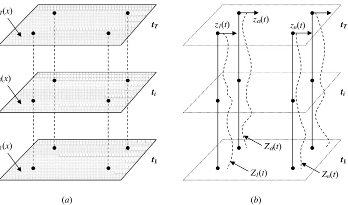
(2) A spatial-temporal process Z(x, t) is viewed as a set of temporally correlated random fields (RF), or a set of spatially correlated time series (TS) depending on which one is the more densely informed. Figure 2-3 illustrates the viewpoint underlying this approach for both cases.
To emphasize, the first approach allows continuous estimation at locations (x) and time (t), whereas the second one gives estimation at a discrete point or a discrete time.
Water resource is also a field of study at which the researches about spatial-temporal variation are relatively active. Stein (1986) presented a mathematical model for spatial-temporal process, for which the observations are modeled as the sum of the random field fixed in time plus a second independent random field that varies both spatially and temporally. This can be considered as a modified form for the first approach presented above. Or and Hanks (1992) also proposed a spatial temporal estimation method to reduce the uncertainty in irrigation management, which basically stems from soil variability and climatic uncertainty. Temporal soil water storage estimates were obtained by the Kalman filter, while spatial estimates were obtained by conditional multivariate normal method. These spatial and temporal estimates were then combined an additional Kalman filter step that considers spatial estimates as a measurements. The separation of spatial uncertainty from temporal uncertainty indicates that this method should be classified in the second approach mentioned above.
The literatures relating to spatial-temporal modeling in the field of Geotechnical engineering are relatively rare and in general focus on the movement of the pore liquid within the soil mass. This
thesis aims to propose a practical approach to introduce spatial-temporal modeling in geotechnical design. Therefore, the temporal variation concerned in the current thesis is for the prediction of temporal soil behavior, such as ground settlement. Due to the fact that the temporal soil behavior basically can be explained by physical models of soil, it is more informative to characterize temporal variation than spatial variation, i.e. the pattern of spatial variation is less likely to be estimated. Therefore, the proposed approach separates spatial variation, which focuses on estimation and interpolation of the soil or model parameters, from the temporal variation, which mainly concerns the prediction of temporal soil behavior at a particular spot of time. In this sense, it can be concluded that the proposed approach shares the similar viewpoint with the second approach presented by Kyriakidis and Journel (1999) for the case that the random process is considered as a set of spatially correlated time series (TS) (see Fig. 2-3(b)), and also similar to the method presented by Or and Hanks (1992). Due to the fact that the proposed formulation can also be transformed to Kalman filter equations (see Appendix A), it can be viewed as a modification of Kalman filter by introducing the spatial correlation into the basic formulation of Kalman filter, which originally deals only with the time and observation updating problem.
Figure 2-1: Uncertainties in geotechnical design.
Figure 2-2: An example of subsoil investigations at two different sites.
Inherent soil variability Measurement uncertainty Statistical uncertainty Transformation uncertainty Design method uncertainty Design stages Uncertainties Soil investigation Transformation to design parameters Design
uncertainties in soil parameter estimates
Aleatory
uncertainty uncertainty Epistemic
Actual properties Measured properties Site A Site B Soil sampling scheme Approximated trend Depth Soil property Depth Soil property
Figure 2-3: Conceptual models of spatial-temporal process when are viewed as (a) a set of random functions (RF) Zi(x), i
= 1, 2, . . . T ; and (b) a set of vectors of time series (TS) Zα(t), α = 1, 2, . . . n (Kyriakidis and Journel 1999). zα(t) z1(t) zn(t) ZT(x) Zi(x) Z1(x) tT ti t1 tT ti t1 Z1(t) Zα(t) Zn(t) (a) (b)