A VARIANT OF THE OUTER APPROXIMATION METHOD FOR GLOBALLY MINIMIZING A CLASS OF COMPOSITE FUNCTIONS

Journal of the Operations Research Society of Japan

Vol. 40, No. 2, June 1997

A VARIANT OF THE OUTER APPROXIMATION METHOD FOR GLOBALLY MINIMIZING A CLASS OF COMPOSITE FUNCTIONS

Takahito Kuno

University of Tsukuba

(Received February 13, 1996; Revised May 20, 1996)

Abstract In this paper, we consider a constrained optimization problem whose objective function is a composition of two functions g : R"

-+

RP and f : RP

-+

R1. We show that a variant of the outer approximation method generates a globally e-minimum point of f o g = f ( g ( - ) ) over a convex set after finitely many iterations, if g is convex and f is continuous and coordinatewise increasing. Preliminary experiments indicate that the proposed algorithm is reasonably practical for two types of multiplicative programs if p is less than four.

1. Introduction

In a series of articles

[5

- 111, Konno et al. studied multiplicative programming problems, whose objective functions can be expressed by the product of some convex functions. Al- though the class is a typical nonconvex program and hence has multiple local minima [IO], one can generate a global minimum rather efficiently if the number of convex functions involved in the product term is much less than that of variables. Tuy [24] and Sniedovich et al. [l91 independently showed that this nice characteristic is mainly due to a low-rank property possessed by multiplicative functions. In other words, minimizing a composition

f o g = f ( g ( - )) of two functions g :

IRn

-+

W

and

f

:

RP

-+

R'

over a convex set A'

C

R"

is possibly as efficient as minimizing the product of p convex functions, if all components of

g are convex on

R"

and

f

is coordinatewise increasing and quasiconcave on

{g(x)

\

X E

X}.

As stated in [11], one of the most important application of multiplicative programs is multiple objective decision making. When several objectives without a common scale need optimizing simultaneously, a handy approach is to optimize the product of these objectives (see e.g. [8]). This approach, however, assumes implicitly that the utility of the decision maker is quasiconcave on his criterion space, though the shape of the utility function is in general difficult to specify except that it is coordinatewise increasing [20].

In this paper, we will develop a method for minimizing

f

o g over a convex set

X

without assuming that f is quasiconcave. More precisely, f is continuous and coordinatewise increasing but needs t o be neither quasiconcave nor quasiconvex on some open set including

{g(x)

1

X E

A'}.

This class of functions

j

o g is a generalization of multiplicative functions and also contains rank-p quasiconcave functions studied by Tuy [24]. We will show that a variant of the outer approximation method can generate a global e-minimum of this nonconvex function after finitely many iterations. Preliminary experiments indicate that the proposed algorithm is reasonably practical for some subclasses when p is less than four,

The author was partially supported by Grand-in-Aid for Scientific Research of the Ministry of Education, Science, Sports and Culture, Grant No. (C)07680447.

246

T,

Kuno

even though n exceeds one hundred. This fact has an important implication in multiple objective decision making, because the number of objectives is usually less than five, and less than three in most practical applications (see e.g.

[ 7 ] ) .

The organization of the paper is as follows: In Section 2, we will transform the problem into a p-dimensional minimization problem whose objective function is

f.

I n Section 3, to solve the resultant problem, we will propose a variant of the outer approximation method. Unlike the usual ones, our algorithm approximates the feasible region by using the union of finitely many rectangles in

RP.

We will discuss possible improvements on the algorithm in Section 4, and report the results of computational experiments in Section 5.

2. Master Problem in the p-Dimensional Space

Suppose a continuous function f : By -+ ]R1 satisfies

for any y G

S,

where

S

is an open subset of

W

and + stands for the nonnegative orthant.

The problem we consider in this paper is to minimize a composition of f and a convex function g : ]Rn -+

IR^

over a convex set X C R", i.e.

minimize

f

o g ( x ) = f ( g ( x ) )

subject to X 6

X.

We assume for simplicity that

X

is compact. Therefore the j t h component g, of g achieves a minimum over

X

a t some X-> for j = 1, .

. .

,

p. Also the objective function of

(P)

has a globally optimal solution in

X,

since the composition of two continuous functions is continuous. We further assume that

Hence it holds for any two feasible solutions X', X" of

(P)

that

under condition (2. l )

.

We first define a univariate function:

for j = 1, ...,p.

Let

Lemma 2.1.

Let

x1

E

X.

If

f

o g(xl)

<

v , then

Proof: Since

gj(x3}

<

gj(xl) for every j, we have

Minimization o f a Composite Function 24 7 Let us introduce a vector y E

W

of additional p variables

y-'S,

and consider the following problem:

minimize f ( y )

subject to X E X,

9(x) - Y

5

07 f-

5

Y

5

U,

T

where

t

= ( t i , . . .

,

l,)"', U = (ui, . . . ,,up) and

Lemma 2.2. Let (X*, y*) be an optimal solution of (2.6). Then X* solves ( P ) .

Proof: Let X' E

X

and assume that

f

o g ( x l )

<

f

o g(x*). Let

xq

= argmin{f o g ( x )

1

X =

xl, .

. .

,

xp}. Then, by the previous lemma, (xq, g ( x q ) ) is feasible to (2.6) and satisfies

We again apply Lemma 2.1 and have

t

<_ g(xl)

<^

U. This is a contradiction, because (X', g ( x f ) ) is feasible to (2.6) and f ( g ( x f ) )

<

f (y*) holds. D

Remark.

For each j = 1,

. . .

,

p, one can compute another upper bound to yj, which may be somewhat better than u j when p

>

2, by solving

maximize{gj(x)

1

X E

X}.

_(2.8)

However, (2.8) is a convex maximization problem and hence is hard to solve in general. In contrast to this, u j can be yielded by an ordinary line search algorithm. Since

f j

is continuous and strictly nondecreasing, computing

u,

= max{t/

1

fj(y) <_ v } amounts to minimizing a certain unimodal function of a single variable.

Let us denote by Z the feasible region of (2.6), i.e.

and let

Y

= {y E

IRP 13x

E

R",

(X, y )

E

Z}.

Then we have a problem in the p-dimensional space: minimize f (y)

subject to y E

V,

which is equivalent to (P) in the following sense:

Theorem 2.3. Let y* be an optimal solution of (MP). Then any X* such that (X*, y*) E Z solves

(P).

Proof: It is obvious that any (X*, y*) E Z is an optimal solution of problem (2.6) if

y*

is optimal to

(MP).

Hence X* solves

(P),

0

248

T.

Kuno

By convexity of g , we see that

Z

is a convex set in

B"

X By. The feasible region V of (MP) is the orthogonal projection of

Z

onto the y-space and hence a convex set in

IV

[18]. We can also see that Y is compact as well as

2.

The above transformation from ( P ) into (MP) is based on a decon~position principle in global optimization

[6,

171.

We

refer to

(MP)

as the master problem of-(-P). If

f

is either convex or (quasi)concave, there are several solution methods for (MP) (e.g. [l, 22, 231). These decomposition algorithms are known to be more promising than solving the original problem directly, when p is much smaller than n. However, in some applications such as multiple objective decision making, the shape of f is often difficult to specify except that it satisfies condition (2.1).

In

the rest of the paper, we will develop an algorithm for solving (MP), in which f is assumed to be neither convex nor (quasi)concave.

3. Outer Approximation Algorithm for the Master Problem

It is straightforward to see from (2.1) that there is a globally optimal solution y* of the master problem

(MP)

among boundary points of the compact convex set

Y.

Hence outer approximation can still work for (MP) even though

f

is not (quasi)concave.

Let us denote

Starting from

Yo

as the initial relaxation of Y, the class of outer approximation algorithms generates a sequence of relaxed problems ( P k ) , k = 0, 1, . . .

,

of the form:

where Y

minimize f ( y ) subject to y E Yk,

Let y k be an optimal solution of (Pk). It follows from (2.1) and (3.2) that y k

if

int Y for every k, where int represents the set of interior points. If y k happens to be a point of V,

then it is a globally optimal solution of (MP) and any X such that ( X ,

yk)

E Z solves the original problem (P) (Theorem 2.3). Otherwise, we need to exclude some portion containing y k from Yk to obtain the next relaxation &+l of Y. The usual procedures construct Yk+l by adding some cutting-plane constraints to the system defining Yk and generate a sequence of polytopes Yk's. When f is (quasi)concave, we need only to search vertices of the polytope for an optimal solution y k of

(Pk).

In our problem, however, such vertices might not provide an optimal solution. We will therefore propose an alternative procedure for excluding y k from Yk in this section. The resultant Yk turns out to be the union of finitely many rectangles in

RP.

3.1. APPROXIMATION

O F T H E FEASIBLE REGION

Suppose an optimal solution y k of the kth relaxed problem ( P k ) is given. Regarding y k as an ideal value of g, let us consider the following minimax problem:

Minimization of a Composite Function 249 where U E

W

is defined in (2.7), and c = ( c i , . . . , c ~ ) ~ is a weighting vector satisfying

CJ

>

O , j = 1, . . . , p , and

E7=icj

= 1.

The objective function

G(-

; y ") is convex and its mininlum point X * ( yk ) can be obtained

if we apply any one of standard algorithms to an equivalent problem: minimize z

subject to X G X, g ( x )

<^

U ,

g j ( x ) - i / C J ^ y ^ , j = l ,

. . . ,

p,

where .;is a scalar variable. It is easy to check that x * ( y k ) is feasible to ( P ) and that

A!

<_

g ( x * ( y k ) )

<

U holds. Hence, by letting y * ( y k ) = g ( x * ( y k ) ), we have a feasible solution y*(y1'} of (UP), which satisfies

Let z ( y ) = G ( x * ( y ) ; y ) and let

-

Y ^

= { y 6

RP

1

c/% -

6)

<

2 ( y k ) , j = l , - . .

,

p}. _(3.5)

Lemma 3.1. Fun,ctzon z :

W

+

R

is convex (and hence con~tinuous), an,d satisfies

Proof: Let y' be an arbitrary point of Y . Then by definition g ( x l ) - y'

<,

0 holds for some

X' 6

-Y,

and hence we have ;(g')

5

m a ~ f i c ~ ~ ~ ( x ' ) - y')l

<:

0 by noting c

>

0. If y k

#

Y,

then no y 6 Y satisfies y y k under condition (2.1) because yk is an optimal solution of a relaxed problem of (P). This implies that there is some index q such that gq(x)

>

y; for any feasible solution X of ( Q ( y k ) ) . Hence the optimal value - s ( y k ) of ( Q ( y k ) ) is positive if Y k

#

y.

Convexity of z is shown as follows: Let y' and y" be any points in W. Then for any

A

G [O, l ] we have

( 1 - A ) z ( y f )

+

A z ( y f f )

= (1 - A ) max, { c j ( g j ( x * ( y f

))

- yi)}

+

A maxj { c j (g j ( x * ( y f ' ) ) - y"}}

2

maxj { ( l - A)cj ( g j ( X * ( Y ' ) ) -

^)

+

\cj ( g j ( X * ( y ' ' ) ) - yy)}

2

m a ~ j { ~ j ( g ~ ( ( l - A ) x * ( y f )

+

A x * ( y f ' ) ) - ( 1 -

Q',

- Ay"}

2

max, { c j (gj(x* ( ( l - A ) y'

+

Ay")) - ( 1 - A ) yi -

Ay;')}

= ;((l - A)yf

+

A y f f ) ,

since cj7s are positive and g-S are convex.

Lemma 3.2. I f y" Y , then

Proof: The first part of (3.7) follows from (3.6). To show the second, choose an arbitrary

( X ' , y') 6

2.

Then we have z ( y k )

5

m a x j { c / g j ( x l ) - t~:)}

5

m a x j { c j ( y i -

$)},

which implies y

vk

for any y 6 V. D

The set

7;.

contains all points y E

RP

which are closer to y k than

y * f y k )

with respect to the weighted rectilinear distance defined by c. These points cannot be feasible, since y * ( y k )

is the closest to yk in the feasible region

Y

(see Figure 4.2 in Section 4.3). Therefore, if we define the k

+

1st relaxation of Y as follows:

a useless portion involving yk are gouged out from

Yk

and no points of

Y

are lost.

If we use the above procedure to generate every relaxed problem, the feasible region

h

of

( P k )

will not be any convex- set but the union of a number of distinct rectangles in

RP,

where

Ik

is some index set and

However, only among the vertices t i 7 s of Ri's exists an optimal solution yk because the ob- jective function

f

has the monotonic property (2.1). Hence we can solve

(Pk)

by performing a t most

IIJ

comparisons:

Let

Ik

denote the subset of indices i

A

such that

l'

F k . If yk is not a point of Y , for each i E

Is,

we have to discard the portion of

R;

included in

Y k .

This can easily be done in the following way:

Let

Jk

be an index set such that

Note that

Jk

is nonempty. Since a gives an upper bound to each feasible solution,

Jk

=

0

implies that Y C Y ' k , which is a contradiction. For each j E Jk let

and define

If we replace

Ri

with

U j e A

Rij

for every i E

J t ,

all the portion of included in

Y\

is discarded, and the next relaxation &.+l is generated as follows:

Thus our algorithm requires no expensive procedures to update the relaxation of

Y,

which contrasts remarkably with the usual cutting-plane algorithms (see e.g. [G] ) .

Some of Rij7s might be redundant in the definition (3.15) of Yt+l. We can remove any

Rij

from (3.15) if

f

>:

ts

for some s E

4

\

. f t . We refer to the rest of f s , together with

f",

i

4

\

fki

as v e r t i c e s of Yk+l by the analogy with convex sets.

3.2. DESCRIPTION O F T H E ALGORITHM

We are now ready to present an outer approximation algorithm for solving the master problem

(MP).

Here e

2

0 stands for a given tolerance.

Minimization o f a Composite Function 251 Algorithm 1.

Step 0. Compute bot,h the bounds 42 and U to g according to (2.3), (2.4) and (2.7), and

define the feasible region Yo = { y 6

W

1

42

5

y

5

U } of the initial relaxed problem ( P o ) . Let k = 0 and go to Step 1.

Step 1. Compute an optimal solution yk of ( P f c ) . Solve a nlinimax problem (QA y k ) ) and let x*(yk} and z ( y k ) be an optimal solution and the optimal value respectively.

Step 2. Let y * ( y k ) = g ( x * ( y k ) ) . If

then stop.

Step 3. Let

YI:

=

{

y E

RP

1

c, ( yj - y^)

<

z ( y k ) , j = 1, . . .

,

p} and update the relaxation of

Y

as Y N I = Yk

\

Fi.

Return to Step 1 with k = k

+

1.

If this algorithm terminates, the stopping criterion (3.16) guarantees the e-optimality of

y * ( y k ) to ( M P ) . By the definition of y * ( y k ) we have ( x * ( y k ) , y * ( y k ) ) E

2.

Hence x * ( y k )

is a globally e-optimal solution of ( P ) in this case. Moreover, we should note that every

x * ( y k ) generated in the course of computation has a certain desirable property in multiple objective programming. Since X * ( y k ) minimizes maxj {cj ( g j ( X ) -

$)}

on for c

>

0,

there are no X E

X

such that g ( x )

<

g ( x * ( y k ) ) . This implies that x*(y1'} is a weakly efficient

solution of a multiple objective program (see e.g. [20]):

'minimize' g (X )

subject to X E X.

Theorem 3.3. Suppose the convex program ( Q ( y ) ) is solved infinite time for any y

_Yo.

Then Algorithm 1 terminates after finitely many iterations i f e

>

0.

If e =

0 ,

Algorithm 1 generates a sequence of points yfc's, every accumulation point of which is a globally optimal solution of

(MP).

Proof: Let us suppose the algorithm does not terminate. Then an infinite sequence { g i }

is generated in the compact set Yo if each ( Q ( y k ) ) is solved in finite time. We can take a subsequence {ykq

\

q = 0, 1, . . .

}

which converges to some point y E

h.

Let us assume the contrary to the assertion, i.e. there exists some constant 0

>

e such that

f

( y * ( y k q ) ) -

f

( Y k q )

2

0, %l- (3.17)

Let h ( y ; y k ) = maxj{cj(i(j -

~ 1 )

- z ( y k ) } . We see from (3.5) that y 6

Yis

if and only if

h ( y ; y k )

<

0.

Then by Lemma 3.2 we have h(ykq+l ; ykq)

2

0

for every q and hence lim h(yfcq+l; yfcq) = lim h(ylq; yfcq) = -z(jj)

2

0

9-a' g - ~

by continuity of z. On the other hand, it follows from (3.6) that z(ykq)

>

0 for every q ,

which also implies z ( y )

>_

0. Consequently, we have

which contradicts assumption (3.17) under condition (2.1). If c

>

0, then (3.16) holds after finitely many iterations and Algorithm 1 terminates. If 6 =

0,

by continuity of f we have

It follows from (3.6) and (3.18) that y 6 V , and hence y is a globally optimal solution of the master problem ( M P ) . D

252

T.

Kuno

4. Some Improvements on the Algorithm

In this section we present two procedures for improving the efficiency of the algorithm developed in Section 3.

4.1. DETERMINATION OF T H E WEIGHTING VECTOR

We have not yet discussed how to determine the weighting vector c of the objective function of (Q(yk)). As shown in Theorem 3.3: Algorithm 1 converges with any fixed c

>

0 and yields an e-optimal solution of (MP) when e

>

0. However, the choice of c will affect the speed of convergence considerably.

From the stopping criterion (3.16), it is desirable to find a feasible solution y of (MP) giving the value f ( y ) as close to

flyk)

as possible. If

f

is differentiable a t y , we have a first-order approximation of f around y k :

Also we have

Hence we can make the difference f l y ) - f ( y k ) rather small by minimizing the right-hand- side of (4.20), i.e.

9f

(Yk)

minimize _{max{- ( g , [ x ) - y,')}

1

_j = 1 , . . .

,

p }

QYi

1

subject to

x

_{X ,}

_{g ( x )}

<

U.

If

/

is continuously differentiable on Yo and V / ( y )

>

0 for all y E Yo, we can use c ( y k ) defined below as the weighting vector of ( ~ ( y ) ) in every iteration of the algorithm:

where e G

B^

is the vector of all ones. In this case, both c and z are continuous on Yo, though z might be no longer convex. Moreover, Lemmas in Section 3 still hold except for the convexity of z . We can therefore prove in just the same way as in the proof of Theorem 3.3 that a subsequence of yk's generated by the algorithm converges to a globally optimal solution of (MP).

If f has no positive gradients a t some points of Yo, we may instead employ

by letting

where

6

is a sufficiently small positive constant and eJ ?E

IV

is the j t h unit vector. Note that

c defined by (4.23) is also continuous and positive valued a t any y k , since f is a continuous function satisfying

(2.1).

Minimization o f a Composite Function 253

4 . 2 . MODIFIED ALGORITHM USING BRANCH-AND-BOUND PROCEDURE

The efficiency of the algorithm will also depend on the number \ I k \ of vertices Ii's of

f i ,

but in particular on the number

17\.j

of those contained in

Y k .

If

Fk

contains only one vertex, say I s , a t most p vertices Is-"s of Yk+i are newly generated. Then we can obtain an optimal solution yk+' of ( P , L + ~ ) only by performing a t most p comparisons if f (f?)'s are sorted beforehand. However, such a favorable situation will not be expected in general so long as we discard

Y k

from the whole of

h.

Suppose Yf, consists of distinct rectangles R i , i E I k , and a vertex Is of Rs = { y E

W

I

P

5

y

5

U } ( S E I k ) provides an optimal solution of ( P k ) . We define the following set:

Yk

=

Yi.

\

(U

R . ) . i#s

L e m m a

4.4.

If

yk

g

Y ,

t h e n

Proof:

Since we are assuming that yk = I s , we have yk

6

Ri for each i

#

s and yk E

rk.

Hence (4.26) follows from Lemma 3.2 and the relation

Yi;

C

yk-

CI

If we discard the portion of

l$

only included in

p',,

then we have an alternative

k

+

1st relaxation of Y:

where

Jk

and RG7s are defined by (3.12) - (3.14). As before, we can remove redundant

rectangles from (4.27) if necessary. This relaxation of

Y

is not so tight as the one based on

(3.8). However, there is still a merit in using it.

If

we update the relaxation of

Y

according

to (4.27)) only one of the vertices is removed and a t most p vertices are newly generated. This leads us to a branching p-tree underlying a branch-and-bound method.

We incorporate the above two procedures into the algorithm. Here e

2

0 is a given tolerance; yO and vO are the incumbent and its objective function value of ( M P ) respectively.

Algorithm

2.

Step

0. Compute the bounds I and U to g according to ( 2 . 3 ) , (2.4) and ( 2 . 7 ) , and define

the feasible region

Yo

= { y E

W

1

l

5

y

5

U } of the initial relaxed problem ( P o ) .

Let

y

= {f.} and initialize the incumbent: yO = U , t1Â =

W ) .

Let

k

= 0 and go to

Step 1.

Step

1. Select yk 6 with the least / ( y k ) and let

y

=

_\

If f is continuously differentiable on

Y9

and V f ( y )

>

0 for all y E

Yo,

then define c ( y k ) according to

( 4 . 2 2 ) . Otherwise, define c ( y k ) according to (4.23) and (4.24). Solve ( ~ ( y " ) ) with the weighting vector c ( y k ) and let x * f y k ) and 2 ( y k ) be an optimal solution and the optimal value respectively.

Step

2. Let y * ( y k ) = g ( x * ( y k ) ) . If f ( y * ( y k ) )

<

v O , then update the incumbent: yO =

y * ( y k ) , t 1 Â =

f

( y * ( y k ) ) . If v0 -

f

( y k )

<

E , then stop.

2 54

T.

Kuno

k k

(i) let yl" = (yl,

.

. .

.

$_,,

y}'

+

:(yk) / c j ,

.

. .

.

and (ii) let =

y

U

{y^} unless yk-'

>

y for some y 6

y.

Return to Step 1 with k = k

+

1.

The following is analogous to Theorem 3.3:

Theorem 4.5. Suppose (Q(y )) i s solved in finite t i m e for any y G

Yo.

T h e n Algorithm 2 terminates after finitely m a n y iterations i f e

>

0. If e = 0, Algorithm 2 generates a sequence

{

yk}, every accumulation point of which is a globally optimal solution of (MP). D

To save the memory required by Algorithm 2, we can employ the depth first rule in

selecting y k from instead of the best bound rule. Since f (yk) gives a lower hound of

/

on the rectangle

R,

= {y E

RP

1

y k

<

- y

<

U } ,

the sign of r0 - / ( y k ) indicates if the

subproblem with

R,

is fathomed or should be branched. When e

>

0, this alteration causes

no trouble though the convergence might be somewhat slower. The procedure presented in Section 4.1 will help to accelerate the convergence. However, we should note that the sequence {yk} might converge to some locally but not globally optimal solution of (MP) when e = 0.

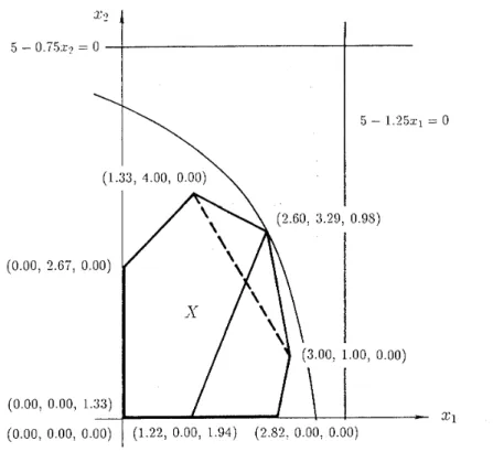
Before concluding this section, let us illustrate Algorithm 2 using a three-dimensional prob-

lem (see Figure 4.1):

minimize (5 - 1 . 2 5 ~ ~ ) (5 - 0 . 7 5 . ~ ~ ) subject to -3x1

+

3x2

+

6x3

<

8, 17x1 - 3x2

+

14x3

<

48, 27x1

+

15x2 - 24x3

<

96, X 1

>

0, X2

>

0, X 3

>

0. Let us define

If we let

S

= {y E

K2

1

y

>

O}, then

/

satisfies condition (2.1) on

S.

Moreover, assumption (2.2) is fulfilled, since

where X' = (3.000, 1.000, 0.000) and x2 = (1.333, 4.000, 0.000) are minimizers of g1 and 92

respectively. Upper bounds of gl and g2 are given as follows:

where v = min{f o g ( x )

1

X = x l , x2} = f o g ( x l ) = 5.313. Thus we have

where

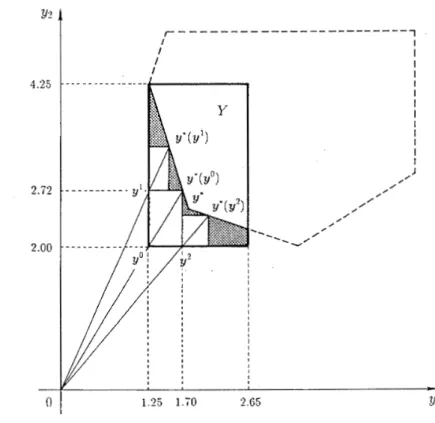
X

is the feasible region of (4.28). Figure 4.2 depicts the feasible region

Y

= {y 6

K

I

3%

E K , (X,

y)

6 Z} of the master problem

(MP).

To solve the master problem, we generate a sequence of its relaxed problems. The feasible

Minimization of a Composite Function

Figure 4.1. Three-dimensional example (4.28) of (P).

is optimal to ( P o ) . Regarding yO as an ideal value of g , we solve a minimax problem:

(Q(vO)l

1

minimize _{subject to} z _X = _E max{cl(3.750 _{X, x i}

₂

_{1.875, x2} - 1.250x1), ~ 2 ( 3 . 0 0 0

_{2 1.000.}

- 0 . 7 5 0 ~ 2 ) }

If we choose cl = 9 f ( y O )

/

9yi = 2.000 and c2 =

my0)

/

8y2 = 1.250, then is optimal to ( Q ( y O ) ) . We also obtain a feasible solution of (MP):

which gives an incumbent value:

According to Step 3 (i), we generate

and let

y

= { y o l , y o 2 } (see Figure 4.2).

Since f ( y o l ) = f ( y o 2 ) = 3.397, both yol and yo2 are optimal to the second relaxed problem ( P l ) . We select an arbitrary y 1 from

y,

say y 1 = yo2. and solve

minimize 2 = max{ci(3.750 - 1.250x1), ~ ( 2 . 2 8 2 - 0.750x2)} subject to X E X, X I

>

1.875, x2

>

1.000,

1.25 1.70 2.65

Figure 4.2. The master problem of (4.28).

where cl = 9f ( y l ) / a y , = 2.718 and c2 = 9 f ( y ' )

/

ay2 = 1.250. Then we have

and let

y

= { y o l , y l l , y12}.

Since f ( g o 1 ) = 3.397 is smaller than f ( y l 1 ) = f ( y 1 2 ) = 4.142, we select yol as y 2 and solve

MY'))

1

minimize _{subject to} X 2 =

c

max{cl(3.302 X, a-1

2

1.875, x2 - 1.250-t-l), c2(3.OOO

2

1.000, - O - T S X ~ ) }

where cl = 9 f ( y 2 )

/

9yl = 2.000 and c2 =

9

f ( y 2 )

/

ay2 = 1.698. Then we have

and let

y

= { y " , y12, y2', y22}.

In the next iteration, we select either y2' or y22 as y 3 , say y3 = y 2 2 , since f ( y 2 ' ) = f ( y 2 2 ) = 4.118

<

f ( y l 1 ) =

f

(y12) = 4.142. Solving ( Q ( Y ~ ) ) , we have

Minimization o f a Composite Function

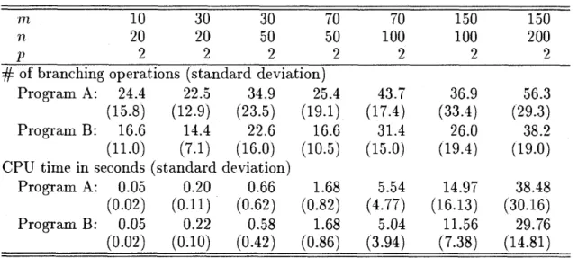
Table 5.1. Comparison between Programs A and B for ( T P l ) when e = 1 0 4

n 2 0 20 50 50 100 100 200

P 2 2 2 2 2 2 9

#

of branching operations (standard deviation)

Program A: 24.4 22.5 34.9 25.4 43.7 36.9 56.3 (15.8) (12.9) (23.5) (19.1) (17.4) (33.4) (29.3)

Program

B:

16.6 14.4 22.6 16.6 31.4 26.0 38.2 (11.0) (7.1) (16.0) (10.5) (15.0) (19.4) (19.0)

CPU time in seconds (standard deviation)

Program A: 0.05 0.20 0.66 1.68 5.54 14.97 38.48 (0.02) (0.11) (0.62) (0.82) (4.77) (16.13) (30.16)

Program B: 0.05 0.22 0.58 1.68 5.04 11.56 29.76

In

the same way, we can generate a sequence of

y k ,

k

=

4 ,

5,

. .

.,

which converges to a point y* = (1.750, 2.530). Hence a globally optimal solution of (4.28) is given by

x * ( y * ) = (2.600, 3.293, 0.983), where the objective function value is f ( g * ) = 4.428. 5. Computational Experiment S

We will report the results of computational experiments on Algorithm 2 presented in the previous section.

We

solved two simple subclasses of

(P):

( T P 1 )

1

minimize

Q ( M

- d J x ) j=l

1

subject to

Ax

<^

b,

X

2

0 , minimize ( M 1 - d T x ) ( M i - d:x)

+

^ ( M j

- d ] _ , x ) ( M j - d J x ) j = 2

1

subject to

Ax

5

b, X

2

0 ,

where A E

K m x n ,

b 6 R*', d j E

K",

j = 1 , . . .

,

p. We drew every component of

A

and dj's randomly from the uniform distribution over [-1.000, 1.0001 and that of

b

from

[0.000, 1.0001, and let

M

= 1.1 n1ax{tlj

1

j

= 1 , . . .

,

p } , M l = 1.1 max{tl1, up},

M j = 1.1 - ~ ~ X { Z . J ~ - ~ , ti,},

j

= 2, . . . , p ,

where cj = max{dJx

1

Ax

5

h, X

>.

O}. While the objective function of ( T P 1 ) is

quasiconcave, that of ( T P 2 ) is in general neither quasiconcave nor quasiconvex [10, 111.

The branching rule we employed was a compromise between the best bound and depth

first rules, i.e. among the last twenty y k ' s of we selected one with the least f ( y k ) when

lyl

>

20, where / ( y k ) =

Wy:

for ( T P 1 ) and

f(yk)

=

+

$-iyf for ( T P 2 ) . Then we tried different weighting vectors for ( Q ( y k ) ) , i.e. c = ( 1 , . . .

,

in Program A and

T.

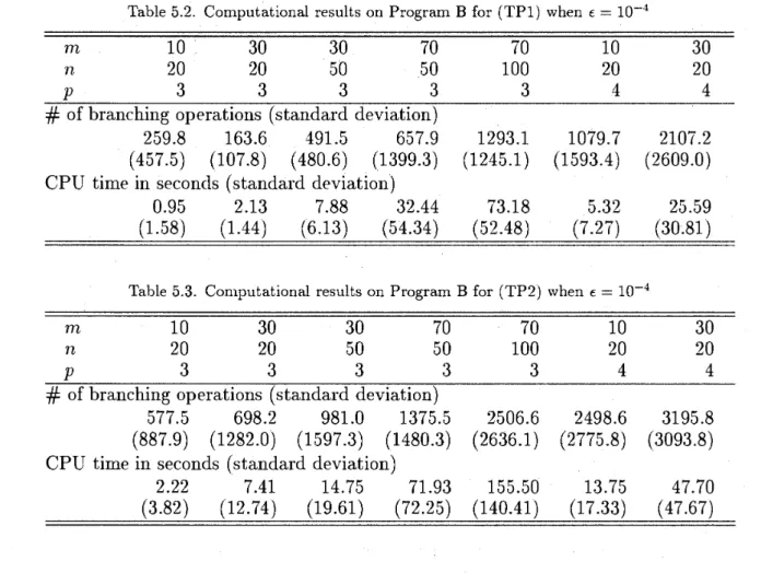
Kuno

Table 5.2. Computational results on Program B for (TP1) when e = l O W 4

m 10 30 30 70 70 10 30

n 20 20 50 50 100 20 20

P

3 3 3 3 3 4 4

#

of branching operations (standard deviation)

259.8 163.6 491.5 657.9 1293.1 1079.7 2107.2

(457.5) (107.8) (480.6) (1399.3) (1245.1) (1593.4) (2609.0)

CPU time in seconds (standard deviation)

0.95 2.13 7.88 32.44 73.18 5.32 25.59

Table 5.3. Computational results on Program B for (TP2) when e = l o 4

m 10 30 30 70 70 10 30

n 20 20 50 50 100 2 0 20

P 3 3 3 3 3 4 4

#

of branching operations (standard deviation)

577.5 698.2 981.0 1375.5 2506.6 2498.6 3195.8

(887.9) (1282.0) (1597.3) (1480.3) (2636.1) (2775.8) (3093.8) CPU time in seconds (standard deviation)

2.22 7.41 14.75 71.93 155.50 13.75 47.70

(3.82) (12.74) (19.61) (72.25) (140.41) (17.33) (47.67)

c = f (yk)

/

v f ( y k ) e in Program

B.

The minimax problem (Q(yk)) of both (TP1) and

(TP2) can be reduced to a linear program. We solved it by using a dual simplex algorithm,

where we took the solution of the preceding (QCy^')) as the starting point. We coded

both Programs A and B in C language and tested them on a microSPARC I1 computer (70

MHz)

.

Table 5.1 shows the comparison between Programs A and B for (TP1) when e = 1 0 4

and p = 2. (Note that (TP1) is equivalent to (TP2) in this case.) The size of (m, n) ranges

from (10, 20) to (150, 200). Tables 5.2 and 5.3 show the results on Program

B

for (TP1) and

(TP2) respectively, when E = lO-*, p = 3, 4 and (m, n ) is between (10, 20) and (70, 100).

Each column of the tables gives the average number of branching operations and CPU time in seconds (and their standard deviations in the brackets) needed for solving ten examples. The number of branching operations corresponds to that of (Q(yk))'s solved in the course of computation.

We see from Table 5.1 that the performance of the algorithm considerably depends on

the choice of the weighting vector. Program

A

requires more branching operations than

Program B. This would affect the total computational time seriously when p

>

2. We also

see from Tables 5.1, 5.2 and 5.3 that Algorithm 2 is very sensitive to the size of p. The

number of branching operations sharply increases as a function of p. However, we should

emphasize that the number is rather insensitive to the size of (m, n ) for each p. This implies

that the total computational time is dominated by that for solving (Qtyk)), i.e. a linear

Minimization o f a Composite Function 259 Since we have experiments with only two subclasses ( T P 1 ) and (TP2). which have special structures handled more efficiently by some existing algorithms (e.g. [12, I s ] ) , no final conclusions can be made about the conlputational performance of our algorithm. However, we can expect from the above preliminary observations that the algorithm will be reasonably practical if p is a small number. say, less than four, and if efficient algorithms for ( Q ( ~ ^ ) ) are available. Computational experiments with more general classes of ( P ) are now under way, whose results will be reported elsewhere.

6. Concluding Remarks

In this paper, we have shown that a globally c-minimum point of a composite function f o g can be obtained in finite time if e

>

0. While nothing is imposed on f regarding convexity or quasiconcavity, the approach requires f to be coordinatewise increasing. Though this may seem to be a rather big assumption, it is quite reasonable in the context of multiple objective decision making, where objectives such as quality, safety, or cost surely do monotonically effect overall utility.

To solve the problem, we have first made a transformation which allows the problem to be solved in the p-dimensional space of variable y replacing

g(x).

This transformation is profitable, especially in decision making, where the number p of decision factors is usually far less than the number n of original variables. We have then developed a variant of the outer approximation method yielding a globally €-optim solution of the p-dimensional problem. Unlike the usual cutting-plane algorithms, the proposed algorithm approximates the feasible region by using the union of finitely many rectangles. This makes the computation for each iteration fairly simpler than those of the usual algorithms. The preliminary experiments suggest that the algorithm is potentially practical for problems with small p.

As we have seen in Section 3.2, the proposed algorithm generates a sequence of weakly efficient solutions of a multiple objective program. Therefore the approach is also considered to be a kind of optimization over the (weakly) efficient set. Since Philip [l61 studied the problem of minimizing a linear function over an efficient set in 1972, problems of this kind have received increasing attention and a number of promising algorithms have been proposed e . g . [2, 3, 4, 5, 211). Like our problem, they belong to global optimization even though the objective functions are linear, because efficient sets are in general not convex 1201.

References

Benders, J .F., "Partitioning procedures for solving mixed variables programming prob- lems", Numerishe Mathematik 4 (1962), 238 - 252.

Benson, H.P., "An algorithm for optimizing over the weakly-efficient set", European Journal of Operational Research 25 (1986), 192 - 199.

Benson, H.P., "An all-linear programming relaxation algorithm for optimizing over the efficient set", Journal of Global Optimization 1 (1991), 83 - 104.

Bolintineanu, S., "Minimization of a quasi-concave function over an efficient set", Math- ematical Programming 6 1 (1993), 89 - 110.

Dauer, J.R. and T.A. Fosnaugh, "Optimization over the efficient set", Journal of Global Optimization 7 (1995), 261 - 277.

Horst, R. and H. Tuy, Global Optimization: Deterministic Approaches, Springer-Verlag (Berlin, 1990).

Keeney,

R.L.

and

H.

Raiffa, Decisions with Multiple Objectives: Preferences and Value Tradeoffs, John Wiley and Sons (New York, 1976).

T.

Kuno

Konno, H. and M. Inori, "Bond port,folio optimization by bilinear fractional program-

ming", Journal of th,e Operations Research Society of Japan 32 (1988). 143 - 158.

Konno,

H.

and T . Kuno, "Generalized linear multiplicative and fractional program-

ming", Annals of the operation,^ Research 25 (1990), 147 - 162.

Konno,

H.

and T. Kimo, "Linear multiplicative programming", Math,ematical Program-

ming 56 (1992), 51 - 64.

Konno, H. and T . Kuno, "Multiplicative programming problems", in

R.

Horst and

P.M. Pardalos (eds.). Handbook of Global Optimization,, Kluwer Academic Publishers (Dortrecht, 1995).

Konno,

H.,

T. Kuno and

Y.

Yajima. "Global minimization of a generalized convex

multiplicative function", Journal of Global Optimization 4 (1994), 47 -- 62.

Konno, H., Y. Yajima and T . Matsui, "Parametric simplex algorithms for solving a

special class of nonconvex minimization problems", Journal of Global Optimization 1 (1991), 65 - 82.

Kuno, T. and

H.

Konno,

"A

parametric successive underestimation method for convex

multiplicative programming problems", Journal of Global Optimization 1 (1991), 267

- 285.

Kuno, T.,

Y.

Yajima and

H.

Konno, "An outer approximation method for minimizing

the product of several convex functions on a convex set", Journal of Global Optimization

3 (1993), 325 - 335.

Philip, J .

,

"Algorithms for the vector maximization problem", Math,ematical Program- ming 2 (1972), 207 - 229.

Lasdon, L.S., Optimization Theory for Large Systems, Macmillan Company (London, 1970).

Rockafellar, R.T., Conevex Analysis, Princeton University Press (Princeton, NJ, 1970).

Sniedovich,

M.,

Macalalag, E. and S. Findlay, "The simplex method as a global opti-

mizer: a c-programming perspective", Journal of Global Optimization 4 (1994), 89 -

109.

Steuer, R.E., Multiple Criteria Optimization: Theory, Computation, and Application,

John Wiley & Sons (NY, 1986).

Thach, P.T., H. Konno and D. Yokota, "Dual approach to minimization on the set of

Pareto-optimal solutions", Journal of Optimization Theory and Applications 88 (1996),

689 - 707.

Thoai, N.V., "A global optimization approach for solving the convex multiplicative

programming problem", Journal of Global Optimization 1 (1991), 145 - 154.

Tuy,

H.,

"Concave minimization under linear constraints with special structure", Op- timization 16 (1985), 335 -- 352.

Tuy,

H.,

"The complementary convex structure in global optimization", Journal of Global Optimization 2 (1992), 21 - 40.

Takahito KUNO:

Institute of Information Sciences and Electronics University of Tsukuba

Tsukuba, Ibaraki 305, Japan