Do Multinationals Use Energy Relatively Efficiently in Malaysian Manufacturing? Additional Evidence for the Early 21st Century

Do Multinationals Use Energy Relatively Efficiently in Malaysian Manufacturing?

Additional Evidence for the Early 21st Century

著者（英） Eric D.  Ramstetter, Shahrazat Binti  Haji Ahmad

journal or

publication title

AGI Working Paper Series

volume 2013‑18

page range 1‑36

year 2013‑06

URL http://id.nii.ac.jp/1270/00000091/

Do Multinationals Use Energy Relatively Efficiently in Malaysian Manufacturing?

Additional Evidence for the Early 21

Century

Eric D. Ramstetter

ICSEAD and Graduate School of Economics, Kyushu University and

Shahrazat Binti Haji Ahmad

Prime Minister’s Office, Government of Malaysia Working Paper Series Vol. 2013-18

June 2013

The views expressed in this publication are those of the author(s) and do not necessarily reflect those of the Institute.

No part of this book may be used reproduced in any manner whatsoever without written permission except in the case of brief quotations embodied in articles and reviews. For information, please write to the Centre.

The International Centre for the Study of East Asian Development, Kitakyushu

Do Multinationals Use Energy Relatively Efficiently in Malaysian Manufacturing?

Additional Evidence for the Early 21

Century Eric D. Ramstetter ([email protected])

International Centre for the Study of East Asian Development and Kyushu University and

Shahrazat Binti Haji Ahmad

Prime Minister’s Office, Government of Malaysia June 2013

Abstract

This paper reexamines energy efficiency differentials between foreign multinational enterprises (MNEs) and local plants in Malaysian manufacturing using data on medium-large plants from the industrial census for 2000 and sample surveys for 2001-2004. Both descriptive statistics and results of econometric estimation indicate that MNEs had a moderate tendency to use relatively little fuel, which was relatively dirty source of energy during this period in Malaysia. MNEs also had a weak tendency to have high electricity intensities as well as low total energy intensities. However, differences in energy intensities between MNEs and local plants were not very pervasive and varied depending on industry and estimation methodology. In short, these results reinforce previous ones, suggesting that both MNEs and local plants generally used energy with similar efficiency during this period in Malaysian manufacturing. The results also suggest that if the goal is to promote greater energy efficiency in Malaysia, there is no reason to discriminate among ownership groups.

Keywords: multinational enterprise, energy efficiency, Malaysia, manufacturing JEL Categories: F23, L60, O53, Q40

Acknowledgement: We are grateful to the Japan Society for the Promotion of Sciences for financial

assistance (grant #22530255 for the project “Ownership and Firm- or Plant-level Energy Efficiency

in Southeast Asia”) and to ICSEAD for logistic support. We thank Kornkarun Cheewatrakoolpong,

Kenichi Imai, Kozo Kiyota, Lin See Yan, Kiichiro Fukusaku, Sadayuki Takii, Siang Leng Wong,

Chih-Hai Yang, and Naoyuki Yoshino for discussing related papers on Indonesia, Malaysia, and

Thailand. Helpful comments were also received from other participants in the Thailand Economic

Conference on 8 June 2012, an ICSEAD Staff Seminar on 11 September 2012, the Asian Economic

Panel on 5-6 October 2012, the 13

International Convention of the East Asian Economic

Association on 19-20 October 2012, a project workshop at ICSEAD on 11 January 2013, and the

10

Pacific Rim Conference of the Western Economic Association International on 14-17 March

2013, as well as from other project participants (Archanun Kohpaiboon and Dionisius A. Narjoko)

and Juthathip Jongwanich. However, the authors are solely responsible for the content of this paper,

including all errors and opinions expressed.

1. Introduction

This paper reexamines the question of whether foreign multinational enterprises (MNEs) used two types of energy (electricity and fuel) and water more efficiently than local plants in Malaysian manufacturing in 2000-2004. In a similar study, Eskeland and Harrison (2003, p.

21) found that “foreign plants are significantly more energy efficient and use cleaner types of energy” than their local peers in Coˆte d’Ivoire, Mexico, and Venezuela. In a related study of provincial data, He (2006) provides evidence that FDI enterprises produce “with higher [SO2] pollution efficiency”, but that stronger environmental regulation has simultaneously, though moderately, deterred FDI among Chinese provinces. Earnhart and Rizal (2006) focus on the effects of financial performance and privatization on environmental performance, but their results indicate foreign ownership was usually an insignificant determinant of pollution in Czech firms. Our previous study of Malaysia (Ramstetter and Haji Ahmad 2012) concluded that MNE ownership was not strongly correlated with energy intensities, with MNEs having a tendency to use relatively little fuel and total energy, and an even weaker tendency to use relatively large amounts of electricity. However, that study omitted an important explanatory variable and made no attempt to address simultaneity issues. Although this study remains unable to address both problems in ideal ways, these results also indicate a weak tendency for MNEs to use relatively little total energy and fuel, and an even weaker tendency to use relatively large amounts of electricity.

These analyses are important because energy consumption generates a large portion of air pollution emitted by manufacturing plants. Improving energy efficiency, or conserving energy, is thus an important way to limit air pollution by manufacturers. For example, if foreign MNEs are more efficient than local plants or firms in host economies as often asserted, they may contribute directly to greater resource efficiency and lower pollution intensity in the host. In Malaysia, electricity is also a relatively clean energy source compared to fuel (mainly oil) consumption. Thus, it is also meaningful to ask if MNE-local differentials in energy intensities vary among relatively clean and dirty energy sources.

The paper first reviews literature related to the resource efficiency of MNEs (Section 2). It

then describes the database used and compares energy intensities in MNEs and local plants (Section 3) and analyzes whether MNE-local differentials persist after accounting for the influences of factor usage, scale, and technical characteristics of plants (Section 4). A methodology similar to that described in Eskeland and Harrison (2003, pp. 16-18) is adopted for this purpose. Section 5 concludes.

2. MNEs, Productivity, and Resource Efficiency in Developing Economies

In recent years, theoretical analyses have highlighted the role of what have been called knowledge-based, intangible assets (terminology from Markusen 1991) in MNEs. The key goals of many theoretical analyses are to explain why the MNE chooses to invest abroad when it (at least) initially has several cost disadvantages compared to local firms, and why the MNE chooses to spread out production across countries rather than concentrate it in one location. Most observers agree that MNEs tend to possess relatively large amounts of technological knowledge and networks, marketing expertise and networks, especially international ones, and generally have relatively sophisticated and capable management.

The first two characteristics are evidenced by relatively high research and development (R&D) intensities (ratios to total sales), relatively large proportions of patent applications and approvals, relatively high advertising-sales ratios, and relatively high dependence on international trade (generally on both exports and imports). Correspondingly, when asking what makes a firm decide to assume the extra costs of investing in a foreign country (compared to the costs of local firms in the host), Dunning (1988) asserted that a firm must first have “ownership advantages” such as those afforded by possession of relatively large amounts intangible assets, as well as “location advantages” and “internalization advantages”

1

Caves (2007) and Dunning and Lundan (2008) provide thorough literature reviews. The work of

Markusen (2002) has also been influential.

before investing.

The important implication is that, if one accepts the idea that MNEs have relatively large amounts of knowledge-based, intangible assets, MNEs will tend to be relatively efficient producers compared to non-MNEs, at least in some respect. And this relatively high efficiency could involve the MNE becoming more resource efficient and/or polluting less as part of efforts to facilitate increased demand among consumers and minimize production costs related to energy and pollution abatement needs. Moreover, because MNEs tend to be relatively R&D- and patent-intensive, and because technologies for clean energy and pollution control often require relatively sophisticated technological inputs, it is logical to expect that MNEs are relatively efficient producers and consumers of goods and services that promote resource efficiency and pollution reduction. For example, evidence from Cole et al.

(2006) suggests that Japanese firms with outward FDI tend to have better environmental performance (pollute less and manage emissions better) than Japanese firms without outward FDI. This finding is consistent with the notion that MNEs are both better able to and more highly motivated to pollute less than non-MNEs in home economies.

Although limited, most of the existing literature on resource efficiency focuses on energy intensities and indicates that MNEs tend to be relatively energy efficient or pollute less, than local counterparts (see introduction). On the other hand, even if MNEs use less energy per unit of output (i.e., they are more energy efficient), MNEs may contribute to higher energy-related pollution volumes if their production levels and energy use are higher with large MNE presence than with relatively low MNE presence, for example. It is also important recognize that analysis of energy intensity or other factor intensity is closely related to productivity analysis because energy intensity is the inverse of a measure of average energy

2

Dunning’s OLI (ownership-location-internalization) paradigm has been influential, but others (Buckley and Casson 1992, Casson 1987, Rugman 1980, 1985) emphasize that the concept of internalization alone can explain the existence of the MNE and its characteristics described here.

3

Cole et al. (2006) also provide evidence that firms with trade are also more likely to have better

environmental performance than firms without trade. Correspondingly, they emphasize that

internationalized firms are more likely to have better environmental performance than others.

productivity.

Although, the theoretical rationale for expecting MNEs to have relatively high productivity is rather convincing, the empirical evidence on productivity differentials between foreign MNEs and local firms in developing economies (which are predominantly non-MNEs) is ambiguous. For example, studies of productivity differentials between foreign MNEs and local non-MNEs in the manufacturing sectors of Malaysia (Oguchi et al 2002, Haji Ahmad 2010), Thailand (Ramstetter 2004, 2006), and Vietnam (Ramstetter and Phan 2008, 2011) suggest that differentials tended to be relatively small and were often statistically insignificant in Thailand and Vietnam. Other evidence from Malaysia (Menon 1998, Oguchi et al. 2002) indicates that the growth of total factor productivity (TFP) was often less rapid in MNEs than non-MNEs. The only known evidence for China also suggests significant differences in both capital- and labor-productivity when all manufacturing firms are combined into one sample (Jefferson and Su 2006). Importantly, the evidence from Malaysia and other Southeast Asian economies cited above suggests that estimates are particularly sensitive to the degree of aggregation, with significant MNE-local productivity differentials becoming infrequent when samples are disaggregated into relatively narrowly defined industry groups with similar products and technologies.

Previous studies of energy intensities in Indonesia (Ramstetter and Narjoko 2012), Thailand (Ramstetter and Kohpaiboon 2012), and Malaysia (Ramstetter and Haji Ahmad 2012) are consistent with the studies of productivity mentioned above. Specifically, they find that MNE-local (Malaysia, Thailand) or MNE-local private (Indonesia) differentials and not pervasive and usually insignificant statistically if the influences of factor use, scale, and technical characteristics of plants are accounted for. As mentioned in the introduction, the primary purpose of this paper is to reexamine the robustness of the results for Malaysia by (1) addressing an omitted variable problem in the previous study and (2) trying to shed light on how simultaneity issues may affect the results obtained.

4

Average productivities (e.g., of capital and labor) are usually measured as ratios of value added to

the input used, but if resources and other intermediate expenditures are considered to be factors of

production, it is more appropriate to measure production as output.

3. The Data and Patterns of Energy Intensities

This study employs the micro data underlying Malaysia’s census of manufacturing plant activity for 2000 (Department of Statistics 2002) and smaller surveys of stratified samples for 2001-2004 (Department of Statistics various years). If samples are limited to plants with viable basic data (i.e., positive values of paid workers, output, worker compensation, and fixed assets), there were 18,799 plants in the 2000 census, but samples were 30-37 percent smaller in 2001-2004.

However, most of the difference between the census and survey samples results from the census’ inclusion of small plants with limited production. For example, if samples are limited to medium-large plants with 20 or more employees and viable basic data the census contained only 8,540 plants while the surveys samples are only 11-13 percent smaller, depending on the year.

Three types of ownership are identified in the Malaysian manufacturing data, majority-local, 50-50 joint ventures, and majority-foreign. In this study, MNEs are thus defined rather narrowly as plants with foreign ownership shares of 50 percent or more.

MNEs are predominantly medium-large plants and medium-large plants differ from small, predominantly local plants in important ways. Thus, it is more meaningful to compare MNEs and non-MNEs in samples of medium-large plants than to include all plants in such comparisons. And although medium-large plants only comprised 56 percent of all plants meeting the above criteria, they accounted for the 98 percent of their production (measured as gross output) or energy expenditures in 2000-2004. Thus, focusing on the sample of medium-large plants excludes very little production or expenditures on energy. In addition, focusing on medium-large plants has the important advantage of removing most outliers from the samples.

When analyzing pollution related issues, it is important to recognize that 12 industries comprising 15 2-digit categories accounted for 92 percent of energy expenditures by Malaysia’s medium-large

5

Unless indicated otherwise, see Ramstetter and Haji Ahmad (2012, Appendix Tables 1a-1j) for the details cited in this and the following two paragraphs.

6

Malaysian data differ somewhat from those for other countries (e.g., Indonesia, Thailand, and

Vietnam) because minority-foreign plants with foreign ownership shares of 10-49 percent, for

example, are usually defined as MNEs.

manufacturing plants in 2000 and 93 percent in all years 2001-2004 (Table 1).

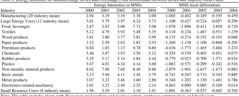
Both of these shares were somewhat larger than these industries’ corresponding share in manufacturing output. Thus, mean ratios of energy expenditures to gross output (i.e., energy intensities) tended to be relatively high in these 12 industries (Table 2). This paper focuses on the analysis of the 12 large energy using industries because they are the largest source of energy-related pollution by manufacturers in Malaysia. MNE shares of expenditures on energy in these 12 industries (36-38 percent in 2000 and 2003-2004 and 42-43 percent in 2001-2002) were often lower than corresponding shares of output.

Thus, energy intensities tended to be lower in MNEs than in local plants. On average in the in these 12 large energy using industries, MNE-local differentials were -1.1 percentage point in 2000, and -0.1 to -0.4 percentage points in subsequent years.

Because energy requirements differ markedly among industries, it is more meaningful to examine industry-level differentials rather than combining data for all 12 industries. For example, electronics-related machinery is a large portion of Malaysian manufacturing and is dominated by MNEs (Table 1). Primarily because of its large size, this industry was the largest energy consumer in all years, accounting for 20 percent of all energy expenditures by medium-large plants in 2000 and 15-17 percent in subsequent years. Shares of this industry were substantially larger if measured in terms output. On the other hand, mean energy intensities were only 2.0-2.5 percent for MNEs in this industry, compared to averages of 3.6-4.2 percent for all 12 industries combined; only petroleum products had lower intensities among MNEs in the 12 large energy using industries (0.6-1.1 percent, Table 2). At the other end of the spectrum, MNE energy intensities were consistently highest in non-metallic mineral products (7.7-8.9 percent).

For the census year (2000), MNEs had lower mean energy intensities than private plants in 10 of the 12 industries, and negative differentials were relatively large (less than -0.3 percentage points) in

7

In this paper, most of these industries (9 of the 12) are defined at the 2-digit level of the Malaysia

Standard Industrial Classification (MSIC), two (rubber and plastics) are the 3 digit components of a

single 2-digit category and one (electronics-related machinery) is a combination of four closely

related 2-digit categories.

nine of those industries (Table 2). However, in 2001-2004, MNEs had lower energy intensities in only about half (6-7) of the industries and relatively large positive differentials (greater than 0.3 percentage points) were almost as common as relatively large negative ones in 2002-2004. In short, these simple calculations suggest that foreign ownership had a relatively weak correlation to total energy intensities in Malaysian manufacturing plants.

The aggregate energy intensities in Table 2 do not reflect the important possibility that MNEs and local plants may consume different energy mixes and thus impart different environmental impacts even if aggregate energy intensities are similar. For example, Eskeland and Harrison (2003) suggest that electricity consumption is cleaner than fuel consumption and find that MNEs tend to consume relatively more electricity than non-MNEs. In Malaysia during this period, electricity generation relied mainly on relatively clean fuels such as natural gas and hydropower. The combined shares of these clean fuels in electricity generation were also much larger than corresponding shares of the primary energy supply in 2000 and 2005. On the other hand, the shares of coal (a relatively dirty fuel) were also much larger than corresponding shares of the primary energy supply and coal’s share of electricity generation increased substantially toward the end of the period under study.

In short, the dominance of gas and hydropower suggests that electricity was a relatively clean source of energy in Malaysia, but increases in the use of coal suggests that differences between electricity and fuel consumption became less pronounced toward the end of the period studied.

In the 12 large energy consuming industries, electricity intensities were always somewhat larger than fuel intensities for both local plants (2.0-2.8 versus 1.9-2.1 percent) and MNEs (2.4-2.9 versus 1.2-1.4 percent; Ramstetter and Haji Ahmad 2012, Appendix Tables 3a-3b). If the 12 industries are combined, fuel intensities were at least 0.6 percentage points lower in MNEs than in local plants in

8

According to Asia Pacific Energy Research Centre (2009), the combined share of natural gas and

hydropower in electricity generation were 88 percent in 2000 and 69 percent in 2005. Corresponding

shares of final energy demand were only 48 and 47 percent, respectively. On the other hand, coal’s

share in electricity generation rose from 7 percent in 2000 to 27 percent in 2005, while its share in the

primary energy supply was 3 and 10 percent, respectively. Oil accounted for another large portion of

the primary energy supply (43 and 39 percent, respectively) but a very small portion of electricity

generation (6 and 4 percent, respectively).

all years (Table 3). Differences in electricity intensities were 0.4 percentage points or smaller in absolute value in all years except 2003, negative in 2000, and positive in 2001-2004. However, here again it is more meaningful to look at the industry-level data. MNE-local differentials in fuel intensities were negative in 10-11 of the 12 industries and relatively large (-0.13 percentage points or lower) in 8-10 industries. Conversely, in 2001-2004, MNE-local differentials in electricity intensities were positive in 8-9 industries and relatively large (greater than 0.13 percentage points) in 7-8 industries. However, in the census year (2000) there were only five positive differentials, and only three relatively large, positive differentials. In short, MNE-local differentials were more pervasive and relatively large for fuels compared to electricity or overall energy in Malaysian manufacturing.

However, these industry-level comparisons may not adequately reflect plant-level variation in energy intensities, and how it is influenced by variation in factor usage (both scale and factor intensities) and other technical characteristics of plants.

4. Energy Intensities and Ownership after Accounting for Factor Usage

This section attempts to examine the relationship between ownership and energy intensities after accounting for plants’ use of other factors and technical characteristics by estimating a model similar to that in Eskeland and Harrison (2003, 16-18). The models are derived by differentiating “a translog approximation to a production function” with respect to the energy input in question and interpreted as “inverse input demands” (p. 16). As a result, energy intensities are a function of the logs of other factor inputs (other intermediate consumption [mainly materials and parts], fixed assets, and labor), the log of a proxy for the quantity of energy used, and factors related to a plant’s technological sophistication.

Unfortunately, the Malaysian data do not include information on the quantity of energy consumed

so real (2000) ringgit values were used as a proxy. Real electricity expenditures were estimated using

the GDP deflator for the electricity and gas industry, and real fuel expenditures calculated using the

producer price index for mineral fuels in the domestic economy (Malaysia, Department of Statistics

2011a, 2011b). Thus, variation of electricity and fuel prices among plants cannot be accounted for, but variation in the electricity-fuel mix is controlled for, as is general inflation. 24 industry-level deflators for manufacturing GDP were used to calculate real values of total intermediate consumption and capital.

This approach is reasonable for intermediate consumption, but can be misleading for capital (fixed assets) because changes in asset prices are not accounted for.

Unfortunately, we know of no deflator or price index for fixed assets in Malaysian manufacturing.

In the Malaysian data, there are two potentially important indicators of technological sophistication, the ratio of research and development (R&D) expenditures to gross output and the share of highly educated workers in the total workforce. Because correlations among these two indicators are surprisingly low, both are included in the model.

The effect of plant ownership is then captured by adding a dummy variable for majority-foreign MNEs. The resulting model for a cross section of i=1…n plants and t=4 or 5 years is:

EP

=a0+a1(LL

)+a2(LK

)+a3(LM

) + a4(LE

)+a5(ES

)+a6(RD

)+a7(DF

) (1) where

DF

=a dummy equal to 1 if plant i, year t is a majority-foreign MNE, 0 otherwise EP

=energy (electricity, or fuel) intensity in plant i, year t (percent)

ES

=share of workers with tertiary education in all workers in plant i, year t (percent)

LE

= natural log of the quantity of energy (electricity, or fuel) purchased by plant i, industry j, year t (real ringgit)

LK

= natural log of the fixed assets less depreciation at yearend in plant i, year t (ringgit) LL

=natural log of the number of workers in plant i, year t

LM

=natural log intermediate expenditures excluding energy (or water) in plant i, year t (ringgit) RD

=ratio of R&D expenditures to gross output in plant i, year t (percent)

If the coefficient a7 is negative, for example, it would mean that MNEs had significantly lower energy intensities after accounting for the influences of other factor usage and the two indicators of

9

These deflators are generally defined at the 2-digit level, but were defined at the 3-digit level or for a combination of 3-digit categories in food and miscellaneous manufacturing and a combination of 2-digit categories for textiles and apparel as well as motor vehicles and other transportation machinery (Malaysia Department of Statistics 2011a).

10

In addition, Eskeland and Harrison (2003) also include machinery imports and plant vintage as

indicators of plant sophistication, but they are not available in the Malaysian data set.

technical sophistication.

As discussed above, energy requirements differ substantially among industries making it highly likely that all slope coefficients will differ among industries. Correspondingly, this paper emphasizes analysis of industry-level regressions. Samples for the petroleum products industry were very small (20-37 plants per year) and plants in this industry are often clear outliers (with unusually high average labor productivity and capital intensity, for example); thus, this industry is omitted from the regression analysis. Comparisons of industry-level regressions to regressions for the 11 sample industries combined are also provided. Because the industry definitions used in this paper are rather aggregate, detailed industry differences in intercepts are allowed for by adding industry dummies at the 3-digit level.

State and year dummies are also included as practical to account for the effects of plant location and annual economic fluctuations on energy intensity.

All estimates use robust standard errors (clustered by plant for random effects estimates) to account for potential heteroscedasticity.

Because it is highly likely that energy intensities are correlated with the choices of other factor inputs, and perhaps with ownership, on the right-hand side of equation (1), simultaneity is a potential concern. In order to investigate the sensitivity of the results to this problem, the model is estimated in in both contemporaneous specifications (as in equation (1)) for 2000-2004 and 2001-2004, and a lagged specification (where all independent variables are lagged one year) for 2001-2004 (Table 4).

This does not solve the simultaneity issue but comparisons among specifications illustrate how severe related problems are like to be. When estimated by pooled OLS, results of estimating the

11

A few of the 2-digit industries are also 3-digit categories. It is common to use more detailed dummies at the 4- or 5-digit level, for example. However, this results in a large number of industry categories and with very few or no MNEs in them. Because this level of disaggregation can make it difficult to interpret the signs on ownership variables (the focus of attention here), more aggregate, 3-digit definitions are used to insure that each industry contains at least 5 or more MNEs.

12

The lack of observations makes it necessary to combine some states when performing some of the

industry-level estimates. In such cases, states with similar population densities and nearby locations

are combined. A previous paper (Ramstetter and Haji Ahmad 2012) also revealed substantial

variation in parameters for two overlapping subperiods (2000-2002 and 2002-2004). Although

potentially important because of the sharp downturn in 2001, these variations are not examined here

because the panels for subperiods are very short (3 years each).

lagged specification resembled the contemporaneous one but there was more divergence of results when the random effects estimator was used.

Results of pooled ordinary least squares (OLS) estimates and random-effects panel estimates are also compared to see if observed differentials are robust to the estimation method. Results of the Breusch and Pagan Lagrangian multiplier test for random effects indicated that the null hypothesis of no random effects could be rejected at the 1 percent level or better in all but one of the samples examined (total energy intensities in food and beverages for the lagged specification in 2001-2004, Appendix Tables 1-3). Thus, the random effects estimates appear preferable econometrically, but the presence of individual effects complicates the interpretation of the key coefficient a7.

In contrast, pooled OLS yields estimates of a7 that are directly comparable with the MNE-local differentials in Tables 2-3 and of paramount concern here. In general, significant MNE-local differentials are more common when pooled OLS is used. Because the economic interpretation of the estimators differs, we are more concerned with showing when the random effects estimates are consistent with pooled OLS results or not, than establishing which estimator is economically superior.

Table 4 presents results of estimating 3 types of energy intensities (total, electricity, and fuel) for 11 of the 12 large energy using industries (excluding petroleum products) combined, and then for each of the 11 industries when estimated individually. If all 11 industries are combined, the model in equation (1) did a better job of explaining variation in total energy intensities (R

between 0.37 and 0.55) than in electricity intensities (R

between 0.16 and 0.21) or fuel intensities (R

between 0.29 and 0.35; Appendix Table 1-3). For fuel and electricity, coefficients on labor, capital, and the energy quantity were always positive and highly significant at the 1 percent level, while coefficients on intermediate expenditures excluding the fuel or water input in question were negative and highly significant. Thus, labor and capital were complements to energy in the production process while

13

Fixed effects panel estimates are not meaningful when investigating MNE-local differentials because ownership is itself a fixed effect for most plants. As a result, fixed effects estimates only reveal the effects of changes in ownership, not ownership-related differences MNEs and local plants.

The random effects estimator yields an estimate of a7 that has elements of the OLS and fixed effects

estimate; estimates individual effects under assumptions of substantial cross section-like variation.

other intermediate consumption was a substitute. When the equation (1) is estimated for total energy, the same results obtain, except that labor’s coefficient becomes insignificant. The skilled-labor variable and R&D intensity variables were generally insignificant, but positive when significant.

Overall, the model in equation (1) performed more or less as expected in plant-level samples such as these, both when all large energy consuming industries were combined and in most industry level samples (see Appendix Tables 1-3 for estimation details).

In the large 11-indutry samples, the coefficient on the MNE dummy was generally insignificant at the standard 5 percent level (Table 4). When significant, the MNE-local differential was negative in the pooled estimates for total energy in 2001-2004 (both) and all pooled OLS estimates for fuel, but positive for pooled OLS estimates of electricity intensities in 2001-2004 (weakly significant at the 10% level in the contemporaneous estimates for 2001-2004). Under assumptions of random effects, the coefficient was never significant for total energy or fuel, but was positive and weakly significant for electricity in 2001-2004 (both contemporaneous and lagged). In other words, the OLS results from large samples of all 11 industries combined suggests a relatively strong tendency for fuel intensities and a weaker tendency for total energy intensities to be relatively low in MNEs compared to non-MNEs. On the other hand, both pooled OLS and random effects estimates indicate a weak tendency for MNEs to have relatively high electricity intensities for 2001-2004, but the relationship is not significant if pooled OLS is used to examine 2000-2004.

At the industry level, coefficients on intermediate material use (negative) and the energy quantity

proxy (positive) were consistently significant and had the same sign as in regressions for all 11

industries combined (Appendix Tables 1-3). However, there were also important differences in slope

coefficient estimates among industries. For example, capital was a significant determinant of total

energy intensities in only 26 (24 of which were positive) of 66 industry-level estimates (3 pooled

OLS and 3 random effects estimates for each of the 11 industries) and labor was significant in only

20 estimates (13 of which were negative). Coefficients on R&D intensities were also significant 22

times, but the direction of this variable’s influence was split; positive in 11 estimates, negative in

another 11. Results for the coefficient on skilled labor were more often negative (11 coefficients) than positive (7 coefficients), suggesting a weak tendency for higher skill intensity to be correlated with greater energy efficiency.

Of the 66 industry-level estimates of coefficients on the foreign ownership dummy, 42 estimates for total energy intensities were insignificant even at the relatively weak 10 percent level (Table 4).

59 coefficients were insignificant for electricity intensities and 37 for fuel intensities. In other words, using relatively good panel data and a basic model that performed more or less as expected, it was usually impossible to reject the null hypothesis that MNEs and local plants used all three energy types similarly even at a weak (10 percent) level of statistical significance. On the other hand, MNE-local differentials were at least weakly significant in 43 percent of the industry-level estimates for fuel intensities, 36 percent of total energy estimates, but only 11 percent of the electricity estimates.

The significance of MNE-local differentials was often inconsistent among samples, specifications, and estimation techniques (Table 4), but there were a few notable exceptions. First in rubber products, MNE-local differentials in total energy intensities were negative and at least weakly significant (at the 10 percent level) for 5 of the 6 estimates (random effects for 2000-2004, contemporaneous being the single exception); differentials were also negative and significant for fuel intensities in 4 of the 6 estimates. Thus, there was some evidence that MNEs used fuel and total energy relatively efficiently in this industry. Second, in metal products, there was equally strong evidence that MNEs used total energy, electricity, and perhaps fuel relatively inefficiently. Differentials were positive and weakly significant in 5 of 6 estimates for total energy and electricity, and in 3 of 6 estimates (all pooled OLS estimates) for fuel. Third, in wood products the coefficient was negative and weakly significant in 4 of 6 cases for total energy and in 3 of 6 estimates for fuel.

Overall, estimated fuel intensity differentials were negative and weakly significant in at least half

of the 6 estimates performed for 5 of the 11 industries, textiles, wood, rubber, basic metals, and

electronics-related machinery (Table 4). Differentials were positive and significant with similar

frequency in food and beverages and metal products. Meanwhile, MNE-local differentials in total energy were negative and at least weakly significant in half or more of the estimates in paper, rubber, and non-metallic mineral products, and positive and significant in metal products. Finally, at the other end of the spectrum, MNE-local differentials in total energy intensities were never weakly significant in chemicals, plastics, or electronics-related machinery, and significant in only one of six estimates for wood and basic metals. For fuel intensities, no significant differences were observed in chemicals and there was one significant difference in plastics. For electricity intensities, other than the 5 significant differences in metal products, there was only one significant differential each in non-metallic mineral products and basic metals; in the other eight industries no weakly significant differences were observed.

At the industry-level, there is a fairly strong tendency for differences that are at least weakly significant when estimated by pooled OLS to become insignificant when estimated by random effects, especially for total energy and fuel intensities (Table 4). For example, pooled OLS suggests negative and weakly significant differentials for fuel intensities in all three estimates for textiles and electronics-related machinery, and positive and significant differentials in metal products, but none of these differentials were even weakly significant when estimated by random effects. In rubber and basic metals, differentials were also negative and highly significant (at the 1 percent level) when estimated by pooled OLS but insignificant in two of the three random effects’ estimates. Finally, in wood, the pooled OLS estimates reveal negative and significant differences, but random effects estimates suggest positive and weakly significant or insignificant differences. In other words, if one assumes that random effects exist and should be accounted for in the estimation, MNE-local differentials have an even greater tendency to be insignificant than if a pooled OLS estimator is assumed to be correct.

On the other hand the differences between estimates of the lagged model and the

contemporaneous model for 2001-2004 are generally not large, especially in industries where

significant MNE-local differentials were often observed (Table 4). For example, coefficients were of

the same sign and at least weakly significant for total energy in paper (OLS), rubber, non-metallic mineral products, and metal products, for electricity in metal products, and for fuel in all industries combined, textiles, wood (OLS), rubber (OLS), basic metals (OLS), metal products, and electronic-related machinery. The starkest discrepancies between the lagged and contemporaneous specifications were observed when fuel intensities were estimated by random effects, with important differences in sign or significance level in food and beverages, wood, paper, rubber, plastics, and basic metals. However, even in these cases, there is no clear pattern in the differences between the lagged and contemporaneous specifications.

5. Conclusions

This paper has examined whether foreign MNEs used energy more efficiently than their local counterparts in a sample of medium-large plants in Malaysian manufacturing during 2000-2004. A literature review highlighted the fact that foreign MNEs are generally assumed to have superior technology to local plants in developing economies like Malaysia. This creates the possibility that they might use inputs like energy and water relatively efficiently. However, the empirical evidence regarding productivity differentials is at best mixed in Malaysia and other Southeast Asian economies.

Both descriptive statistics and results of econometric estimation are consistent with this mixed

picture. They suggest that the relationship between MNE ownership and energy intensities was

relatively weak during this period in Malaysia. The strongest correlations were observed for fuel

intensities, with MNEs having a moderate tendency to use relatively little of this relatively dirty

source of energy. MNEs also had a weak tendency to have high electricity intensities as well as low

total energy intensities. However, differences in energy between MNEs and local plants were not

pervasive. These results are consistent with the notion that Malaysia is a middle-income economy

and where energy efficiency level that is similar in both local plants and MNEs. The results also

suggest that both MNEs and local plants react to Malaysian policies affecting energy prices and

energy-related pollution in a similar manner. This evidence also suggests it not meaningful for policy makers that are concerned with energy efficiency to distinguish between MNEs and local plants in Malaysian manufacturing.

However, these results need to be interpreted with caution for at least three reasons. First, the proxy for the quantities of fuel and electricity (and thus total energy) do not account for plant-level variation in energy prices. Second, the estimation techniques used in this paper do not adequately account for potential simultaneity. However, the sensitivity of the results to this potential problem has been investigated by lagging all independent variables, and the lagged and contemporaneous specifications generally yielded similar results. Third, it is possible that foreign MNE presence may affect energy intensities in local plants, though the existing evidence suggests that this relationship was also relatively weak in Malaysian manufacturing during this period (Ramstetter and Haji Ahmad 2013).

References

Asia Pacific Energy Research Centre (2009), APEC Energy Demand and Supply Outlook 4

Edition Economy Review, Tokyo: Institute of Energy Economics.

Buckley, Peter J. and Mark Casson (1992), The Future of the Multinational Enterprise, 2nd Edition.

London: Macmillan.

Caves, Richard E. (2007), Multinational Enterprise and Economic Analysis, Cambridge, UK:

Cambridge University Press.

Cole, Matthew A., Robert J.R. Elliott, and Kenichi Shimamoto (2006), "Globalization, firm-level characteristics and environmental management: A study of Japan" Ecological Economics, 59(2), 312-323.

Department of Statistics (2002), Census of Manufacturing Industries 2001 [2000 data]. Kuala Lumpur: Department of Statistics.

Department of Statistics (2010), Malaysia Economic Statistics-Time Series 2009, Kuala Lumpur:

Department of Statistics.

Department of Statistics (various years), Annual Survey of Manufacturing Industries, 2002-2005

issues [2001-2004 data], Kuala Lumpur: Department of Statistics.

Dunning, John H. (1988), Explaining International Production. London: Unwin Hyman.

Dunning, John H. and Sarianna M. Lundan (2008), Multinationals and the Global Economy, 2

Ed., London: Edward Elgar.

Eskeland, Gunnar S. and Ann E. Harrison, (2003), "Moving to greener pastures? Multinationals and the pollution haven hypothesis", Journal of Development Economics, 70(1), 1-23.

Haji Ahmad, Shahrazat Binti (2010), “A Quantitative Study on the Productivity of the Manufacturing Industry in Malaysia”, Ph.D. Dissertation, University of Kitakyushu. Ch. 6.

He, Jin (2006), "Pollution haven hypothesis and environmental impacts of foreign direct investment:

The case of industrial emission of sulfur dioxide (SO2) in Chinese provinces", Ecological Economics, 60(1), 228-245.

Markusen, James R. (1991), "The Theory of the Multinational Enterprise: A Common Analytical Framework," in Eric D. Ramstetter, ed., Direct Foreign Investment in Asia's Developing Economies and Structural Change in the Asia-Pacific Region, Boulder, Co: Westview Press, pp.

11-32.

Markusen, James R. (2002), Multinational Firms and the Theory of International Trade, Cambridge:

MIT Press.

Menon, Jayant (1998) "Total Factor Productivity Growth in Foreign and Domestic Firms in Malaysian Manufacturing", Journal of Asian Economics, 9(2): 251-280.

Oguchi, Noriyoshi, Nor Aini Mohd. Amdzah, Zainon Bakar, Rauzah Zainal Abidin, and Mazlina Shafii (2002) "Productivity of Foreign and Domestic Firms in Malaysian Manufacturing Industry", Asian Economic Journal, 16(3), 215-228.

Ramstetter, Eric D. (2004) "Labor productivity, wages, nationality, and foreign ownership shares in Thai manufacturing, 1996-2000", Journal of Asian Economics, 14(6): 861-884.

Ramstetter, Eric D. (2006) “Are Productivity Differentials Important in Thai Manufacturing?” in Eric D. Ramstetter and Fredrik Sjöholm, eds., Multinational Corporations in Indonesia and Thailand:

Wages, Productivity, and Exports. Hampshire, UK: Palgrave Macmillan, pp. 114-142.

Ramstetter, Eric D. (2011) “Ranking Locations for Japan’s Manufacturing Multinationals in Asia: A Literature Survey Illustrated with Indexes”, Asian Economic Journal, 25(2), 197-226.

Ramstetter, Eric D. (2012). “Foreign Multinationals in East Asia’s Large Developing Economies”, Working Paper 2012-06, Kitakyushu: International Centre for the Study of East Asian Development (http://file.icsead.or.jp/user03/1049_238.pdf).

Ramstetter, Eric D. and Shahrazat Binti Haji Ahmad (2012), “Foreign Multinationals in Malaysian

Manufacturing after the Crisis”, Thammasat Economic Journal, 29(4), 124-160.

Ramstetter, Eric D. and Shahrazat Binti Haji Ahmad (2012), “Do Multinationals Use Water and Energy Relatively Efficiently in Malaysian Manufacturing”, Working Paper 2012-13, Kitakyushu:

International Centre for the Study of East Asian Development (http://file.icsead.or.jp/user04/886_224_20121116114821.pdf).

Ramstetter, Eric D. and Shahrazat Binti Haji Ahmad (2013), “Does Multinational Presence Affect Energy Efficiency in Malaysia’s Local Manufacturing Plants?”, Working Paper 2013-16, Kitakyushu: International Centre for the Study of East Asian Development , forthcoming.

Ramstetter, Eric D. and Archanun Kohpaiboon (2012), “Foreign Ownership and Energy Efficiency in Thai Manufacturing Plants”, Working Paper 2012-12, Kitakyushu: International Centre for the Study of East Asian Development (http://file.icsead.or.jp/user04/886_226.pdf).

Ramstetter, Eric D. and Dionisius Narjoko (2012), “Ownership and Energy Efficiency in Indonesia’s Manufacturing Plants”, Working Paper 2012-14, Kitakyushu: International Centre for the Study of East Asian Development (http://file.icsead.or.jp/user04/886_222_20130108095037.pdf).

Ramstetter, Eric D. and Phan Minh Ngoc (2008), “Productivity, Ownership, and Producer Concentration in Vietnam's Manufacturing Industries”, Working Paper 2008-04, Kitakyushu:

International Centre for the Study of East Asian Development (http://file.icsead.or.jp/user04/833_212.pdf).

Ramstetter, Eric D. and Phan Minh Ngoc (2013), "Productivity, Ownership, and Producer Concentration in Transition: Further Evidence from Vietnamese Manufacturing", Journal of Asian Economics, 25(1): 28-42.

Rugman, Alan M., (1980) "Internalization as a General Theory of Foreign Direct Investment: A Re-Appraisal of the Literature," Weltwirtschaftliches Archiv, 116(2), 365-379.

Rugman, Alan M. (1985) "Internalization is Still a General Theory of Foreign Direct Investment,"

Weltwirtschaftliches Archiv, 121(3), 570-575.

Table 1: Energy Expenditures in Medium-Large Plants with Viable Data and MNE shares

Expenditures (RM millions) MNE shares (%)

Industry 2000 2001 2002 2003 2004 2000 2001 2002 2003 2004

Manufacturing 9,873 8,904 10,311 11,104 12,226 36 42 42 36 38

Large Energy Users 9,132 8,244 9,546 10,362 11,345 36 42 43 36 38

Food, beverages 950 889 955 1,074 1,167 21 23 24 20 21

Textiles 522 486 487 430 466 72 74 72 72 76

Wood products 439 411 420 485 538 16 17 17 16 20

Paper products 392 297 314 330 363 9 14 9 9 10

Petroleum products 315 320 500 745 808 32 74 70 14 14

Chemicals 1,057 1,033 1,347 1,507 1,779 54 58 56 45 50

Rubber products 575 558 575 644 664 31 33 34 33 33

Plastics 434 379 523 534 489 21 29 33 38 31

Non-metallic mineral products 1,308 1,341 1,392 1,369 1,516 23 23 25 28 29

Basic metals 830 886 1,022 1,285 1,234 14 13 14 13 10

Metal products 327 231 266 289 302 39 45 41 45 35

Electronics-related machinery 1,983 1,413 1,745 1,670 2,019 57 81 76 74 77

Small Energy Users 741 661 766 741 882 31 33 31 30 31

Tobacco 27 29 35 25 27 29 26 21 21 23

Apparel 61 50 66 61 58 29 39 51 43 43

Leather, footwear 12 8 9 8 14 36 31 22 28 40

Publishing 67 59 75 69 80 10 11 10 12 10

General machinery 173 165 186 168 207 67 67 59 54 61

Motor vehicles 153 150 176 173 230 12 10 7 17 12

Other transport equipment 63 58 60 69 77 19 19 19 17 23

Miscellaneous & recycling 185 142 160 167 189 27 33 32 28 30

Note: This table includes plants with 20 or more paid workers and positive output, employee compensation, and fixed assets.

Source: Author's compilations from micro data underlying Department of Statistics (2002, various years)

Table 2: Energy Intensities in Medium-Large MNEs and Percentage Point Differentials between MNEs and Majority-local Plants Energy Intensities in MNEs MNE-local differentials

Industry 2000 2001 2002 2003 2004 2000 2001 2002 2003 2004

Manufacturing (20 industry mean) 2.94 3.19 3.19 3.38 3.00 -1.065 -0.402 -0.349 -0.195 -0.459 Large Energy Users (12 industry mean) 3.61 3.79 3.97 4.24 3.73 -1.108 -0.427 -0.224 -0.057 -0.296

Food, beverages 2.67 2.83 3.08 7.72 3.08 -1.070 -1.096 -0.411 3.858 -0.720

Textiles 5.12 4.79 5.92 5.48 5.35 0.118 0.234 1.467 0.551 1.239

Wood products 3.61 3.80 3.77 3.81 3.99 -0.115 -0.274 -0.193 -0.191 -0.068

Paper products 2.52 2.59 2.62 2.83 2.93 -1.260 -1.138 -1.100 -0.860 -0.205

Petroleum products 0.84 1.03 1.13 0.78 0.60 -4.636 -1.773 -1.465 -3.404 -3.233

Chemicals 3.46 3.87 3.93 3.56 3.12 -0.354 0.539 0.403 0.451 0.075

Rubber products 5.25 5.17 5.14 4.84 4.44 -0.779 -0.923 -0.709 -1.371 -0.924

Plastics 3.67 4.01 4.34 4.14 3.68 -1.063 -0.571 -0.209 -0.242 -0.516

Non-metallic mineral products 8.02 7.90 7.65 8.40 8.86 -2.879 -1.961 -2.617 -1.473 -0.882

Basic metals 3.13 3.96 4.11 3.45 3.79 -0.741 0.543 0.733 0.345 0.885

Metal products 3.07 3.32 3.46 3.60 2.80 0.346 1.203 1.330 1.481 0.786

Electronics-related machinery 2.01 2.23 2.49 2.25 2.14 -0.863 0.090 0.085 0.169 0.014 Small Resource Users (8 industry mean) 1.94 2.29 2.01 2.10 1.91 -1.001 -0.363 -0.537 -0.402 -0.705 Note: This table includes plants with 20 or more paid workers and positive output, employee compensation, and fixed assets.

Source: Author's compilations from micro data underlying Department of Statistics (2002, various years)

Table 3: Percentage Point Differentials of Electricity and Fuel Intensities between MNEs and Majority-local Plants

Electricity intensities Fuel intensities

Industry 2000 2001 2002 2003 2004 2000 2001 2002 2003 2004

Manufacturing (20 indutry-level mean) -0.338 0.296 0.326 0.504 0.242 -0.727 -0.697 -0.674 -0.699 -0.701 Large Resource Users (12 industry mean) -0.402 0.346 0.428 0.709 0.327 -0.706 -0.773 -0.652 -0.766 -0.623 Food, beverages -0.559 -0.475 -0.081 4.030 -0.368 -0.511 -0.621 -0.331 -0.172 -0.352

Textiles 0.524 0.895 1.383 1.183 1.619 -0.405 -0.661 0.084 -0.632 -0.379

Wood products 0.647 0.788 0.611 0.594 0.351 -0.762 -1.062 -0.804 -0.785 -0.418

Paper products -0.607 -0.221 -0.145 -0.082 0.285 -0.653 -0.917 -0.955 -0.779 -0.490 Petroleum products -3.178 -0.421 -0.062 -0.681 -0.521 -1.458 -1.353 -1.402 -2.722 -2.712

Chemicals -0.386 0.451 0.483 0.454 0.102 0.032 0.087 -0.079 -0.003 -0.027

Rubber products 0.052 0.185 0.057 -0.051 0.169 -0.831 -1.108 -0.766 -1.321 -1.094

Plastics -0.784 -0.406 -0.082 -0.133 -0.309 -0.279 -0.165 -0.126 -0.109 -0.207

Non-metallic mineral products 0.386 1.086 0.674 1.179 0.845 -3.265 -3.047 -3.291 -2.653 -1.728

Basic metals -0.226 0.806 0.869 0.611 0.711 -0.515 -0.263 -0.136 -0.266 0.174

Metal products 0.058 1.167 1.176 1.185 0.822 0.288 0.036 0.154 0.295 -0.036

Electronics-related machinery -0.745 0.291 0.255 0.218 0.221 -0.118 -0.201 -0.170 -0.049 -0.208 Small Resource Users (8 industry mean) -0.243 0.221 0.172 0.197 0.114 -0.758 -0.584 -0.708 -0.599 -0.819 Note: This table includes plants with 20 or more paid workers and positive output, employee compensation, and fixed assets.

Source: Author's compilations from micro data underlying Department of Statistics (2002, various years)

Energy intensity, industry 2001-2004 2001-2004 2000-2004 2001-2004 2001-2004 2000-2004 11 industries combined -0.0595 -0.3063 a -0.3355 a 0.0210 -0.0734 -0.1104 Food & beverages 1.2950 -0.3863 a -0.4405 a 1.2950 -0.1474 -0.2509 c

Textiles -0.4640 -0.5542 b -0.5353 b -0.4283 -0.4807 -0.0274

Wood products -0.3231 b -0.1906 -0.1790 0.0753 -0.0011 -0.0032

Paper products -0.5580 b -0.7982 a -0.7401 a -0.0400 -0.5895 c -0.4283

Chemicals -0.0724 -0.1321 -0.1913 0.0234 -0.2470 -0.2189

Rubber products -0.8654 a -0.8248 a -0.7692 a -0.7553 b -0.6349 b -0.4385

Plastics 0.1315 0.0885 -0.0879 0.1025 0.1863 -0.1973

Non-metallic mineral products -0.9966 b -1.0201 b -1.0268 a -0.5862 0.1302 0.4549

Basic metals 0.1854 -0.0555 -0.0715 a 0.3161 -0.1265 0.0435

Metal products 0.6204 a 0.5362 a 0.3676 a 0.4906 b 0.3119 b 0.1334 Electronics-related machinery -0.0548 0.0685 -0.0904 0.0853 0.0882 -0.1033 11 industries combined 0.3537 b 0.3145 c 0.1403 0.3427 c 0.3180 c 0.0784

Food & beverages 1.6106 1.4786 1.0614 1.6387 1.5487 1.0460

Textiles 0.0700 0.0634 -0.0673 0.1925 0.1496 0.0604

Wood products 0.0419 0.1839 0.1887 -0.0806 0.2004 0.2571

Paper products 0.1884 -0.0724 -0.1934 0.0257 -0.1248 -0.1716

Chemicals 0.0076 -0.0110 -0.0690 0.1622 0.0009 -0.0811

Rubber products 0.0231 -0.0096 -0.0281 0.0945 -0.0428 0.0426

Plastics 0.2424 0.1708 0.0014 0.1943 0.2090 -0.0978

Non-metallic mineral products -0.1565 -0.2916 -0.3056 c -0.1215 0.1632 0.0550

Basic metals 0.3434 0.1762 0.1127 0.5261 b 0.0381 0.0731

Metal products 0.4088 a 0.4368 a 0.2110 b 0.3188 a 0.3228 a -0.0115 Electronics-related machinery 0.0598 0.1662 -0.0472 0.0730 0.1605 -0.1295 11 industries combined -0.1262 b -0.1097 b -0.1294 a -0.0485 0.0142 -0.0165 Food & beverages 0.2402 c 0.1776 0.1193 0.1429 0.2626 b 0.0789

Textiles -0.5862 b -0.5436 b -0.4921 b -0.3875 -0.4752 -0.0118

Wood products -0.4045 a -0.2582 b -0.3221 a 0.3701 c -0.2869 -0.1903 Paper products -0.0951 -0.1581 -0.1915 c -0.0618 -0.1631 c -0.2031 b

Chemicals 0.1446 0.0239 0.0385 -0.0687 -0.1061 -0.1160

Rubber products -0.9546 a -0.8778 a -0.8447 a -0.6285 b -0.1864 -0.0546

Plastics 0.0145 0.0981 0.0516 -0.0515 0.1641 b -0.0089

Non-metallic mineral products -0.9023 c -0.7608 -0.8997 b -0.2943 0.1384 0.0037 Basic metals -0.3769 a -0.3386 a -0.3795 a -0.2336 c -0.1753 -0.1495

Metal products 0.2913 a 0.2708 a 0.2507 a 0.1098 0.0953 0.1254

Electronics-related machinery -0.0813 a -0.0531 c -0.0478 b 0.0164 -0.0367 0.0108 Notes: a=signficant at the 1% level, b=significant at the 5% level, c=significant at the 10% level;

coefficients from pooled OLS estimates equation (1) that also include industry and region dummies (see text for defintions); other slope coefficients and equation details available from authors.

Lagged Contemporaneous

FUEL INTENSITIES

Table 4: Estimates of Multinational-Local Energy Differentials in Malaysian Manufacturing after Controlling for Factor Inputs, Skilled Labor Shares, and R&D Intensities (percentage points)

Lagged Contemporaneous TOTAL ENERGY INTENSITIES

ELECTRICITY INTENSITIES

Pooled OLS Random Effects

Industry, independent variable, 2001-2004 2001-2004 2000-2004 2001-2004 2001-2004 2000-2004

indicator Coeff. P-value Coeff. P-value Coeff. P-value Coeff. P-value Coeff. P-value Coeff. P-value

LK

0.0987 0.00 0.0999 0.00 0.1061 0.00 0.1186 0.00 0.0604 0.01 0.0833 0.00

LL

0.0603 0.41 0.0082 0.90 0.0039 0.94 0.1610 0.13 0.1590 0.10 0.1030 0.22

LM

-2.3951 0.00 -2.4457 0.00 -2.4818 0.00 -1.9823 0.00 -2.1009 0.00 -2.0740 0.00

LE

2.2639 0.00 2.3587 0.00 2.3783 0.00 1.7248 0.00 1.8631 0.00 1.8232 0.00

ES

-0.0032 0.23 -0.0019 0.44 -0.0006 0.77 -0.0023 0.43 0.0020 0.50 0.0011 0.68

RD

0.0297 0.31 0.0425 0.07 0.0451 0.03 0.0416 0.17 0.0440 0.27 0.0282 0.40

DF

-0.0595 0.77 -0.3063 0.00 -0.3355 0.00 0.0210 0.91 -0.0734 0.38 -0.1104 0.12

Observations/R

17,432 0.38 21,341 0.55 27,373 0.54 17,432 0.37 21,341 0.55 27,373 0.53

Breusch-Pagan test - - - - - - 2,521.66 0.00 10,121 0.00 13,891 0.00

LK

0.1210 0.13 0.2075 0.00 0.2000 0.00 0.1210 0.17 0.1335 0.01 0.0979 0.02

LL

-0.4055 0.05 -0.1225 0.31 -0.1675 0.10 -0.4055 0.09 0.3410 0.07 0.1644 0.32

LM

-2.7528 0.00 -2.7716 0.00 -2.8041 0.00 -2.7528 0.00 -2.2400 0.00 -2.1623 0.00

LE

2.5390 0.00 2.5439 0.00 2.5639 0.00 2.5390 0.00 1.7186 0.00 1.7511 0.00

ES

-0.0133 0.17 -0.0084 0.08 -0.0019 0.69 -0.0133 0.22 0.0027 0.61 0.0064 0.16

RD

-0.0138 0.80 -0.0008 0.97 -0.0004 0.99 -0.0138 0.80 -0.0099 0.15 -0.0132 0.10

DF

1.2950 0.43 -0.3863 0.00 -0.4405 0.00 1.2950 0.43 -0.1474 0.35 -0.2509 0.06

Observations/R

3,771 0.18 4,716 0.59 5,913 0.59 3,771 0.18 4,716 0.57 5,913 0.58

Breusch-Pagan test - - - - - - 0.00 1.00 2,186.69 0.00 3,661.14 0.00

LK

-0.1521 0.04 -0.0976 0.51 -0.1163 0.35 -0.0034 0.96 -0.0213 0.86 -0.0462 0.56

LL

-0.5560 0.03 -0.1489 0.61 -0.2625 0.31 -0.4267 0.20 0.2288 0.54 0.0084 0.98

LM

-1.6817 0.00 -1.4599 0.00 -1.6311 0.00 -1.4602 0.00 -1.0542 0.00 -1.0218 0.00

LE

2.6335 0.00 1.9891 0.00 2.1897 0.00 2.1396 0.00 1.2790 0.00 1.2588 0.00

ES

0.0091 0.60 0.0338 0.05 0.0394 0.05 0.0070 0.74 0.0305 0.15 0.0170 0.31

RD

0.1780 0.15 0.4546 0.00 0.2327 0.05 0.1158 0.26 -0.2329 0.01 -0.0567 0.57

DF

-0.4640 0.15 -0.5542 0.04 -0.5353 0.03 -0.4283 0.31 -0.4807 0.26 -0.0274 0.94

Observations/R

571 0.62 667 0.60 862 0.56 571 0.61 667 0.55 862 0.50

Breusch-Pagan test - - - - - - 52.52 0.00 136.68 0.00 163.06 0.00

11 LARGE ENERGY USING INDUSTRIES COMBINED

FOOD AND BEVERAGES

TEXTILES

Appendix Table 1: Multinational-Local Differentials in Energy Intensities and Other Details from Estimates of Equation (1)

Pooled OLS Random Effects

Lagged Contemporaneous Lagged Contemporaneous

Industry, independent variable, 2001-2004 2001-2004 2000-2004 2001-2004 2001-2004 2000-2004

indicator Coeff. P-value Coeff. P-value Coeff. P-value Coeff. P-value Coeff. P-value Coeff. P-value

LK

0.2869 0.00 0.2098 0.00 0.1929 0.00 0.2104 0.03 0.1864 0.07 0.1867 0.01

LL

0.6310 0.00 0.5063 0.02 0.5260 0.00 0.2870 0.28 0.6499 0.04 0.5267 0.07

LM

-2.0923 0.00 -2.3002 0.00 -2.2753 0.00 -0.8827 0.00 -2.4068 0.00 -2.2795 0.00

LE

1.2148 0.00 1.5262 0.00 1.5333 0.00 0.3094 0.01 1.2416 0.00 1.4172 0.00

ES

0.0168 0.10 0.0211 0.01 0.0262 0.00 0.0017 0.84 0.0036 0.78 0.0177 0.03

RD

-0.1220 0.48 -0.0560 0.60 0.0737 0.70 0.0202 0.93 -0.0624 0.15 0.0929 0.57

DF

-0.3231 0.03 -0.1906 0.13 -0.1790 0.13 0.0753 0.76 -0.0011 1.00 -0.0032 0.99

Observations/R

2,091 0.24 2,409 0.33 3,154 0.36 2,091 0.15 2,409 0.31 3,154 0.35

Breusch-Pagan test - - - - - - 134.15 0.00 245.94 0.00 436.61 0.00

LK

-0.0890 0.54 -0.0276 0.73 0.0074 0.92 -0.1200 0.15 0.0203 0.79 0.0358 0.64

LL

-0.6661 0.06 -1.2920 0.00 -0.8824 0.00 0.2229 0.52 -0.6457 0.03 -0.5728 0.01

LM

-3.0489 0.00 -2.7611 0.00 -2.9235 0.00 -2.0552 0.00 -2.1010 0.00 -2.3118 0.00

LE

3.2316 0.00 3.4504 0.00 3.2615 0.00 1.5690 0.00 2.3253 0.00 2.4181 0.00

ES

-0.0404 0.01 -0.0474 0.00 -0.0386 0.00 -0.0009 0.90 -0.0097 0.10 -0.0029 0.76

RD

-0.3948 0.14 -0.1601 0.57 -0.0175 0.95 -0.0890 0.57 0.2127 0.48 0.1182 0.60

DF

-0.5580 0.05 -0.7982 0.00 -0.7401 0.00 -0.0400 0.86 -0.5895 0.06 -0.4283 0.11

Observations/R

757 0.57 923 0.62 1,190 0.63 757 0.45 923 0.57 1,190 0.59

Breusch-Pagan test - - - - - - 285.36 0.00 400.01 0.00 606.96 0.00

LK

0.1883 0.03 0.1461 0.09 0.1801 0.05 0.1460 0.20 -0.0033 0.97 0.0695 0.41

LL

-0.2944 0.26 -0.3519 0.13 -0.3875 0.04 0.4535 0.17 -0.2357 0.51 -0.1036 0.73

LM

-2.3041 0.00 -2.3296 0.00 -2.3652 0.00 -1.5769 0.00 -2.3449 0.00 -2.1539 0.00

LE

2.2107 0.00 2.3033 0.00 2.3300 0.00 1.0107 0.00 2.4482 0.00 2.1316 0.00

ES

-0.0007 0.94 0.0011 0.89 -0.0018 0.79 0.0033 0.72 0.0043 0.65 -0.0046 0.56

RD

-0.2673 0.01 -0.2772 0.01 -0.2783 0.00 -0.0597 0.19 -0.0802 0.09 -0.4178 0.23

DF

-0.0724 0.78 -0.1321 0.51 -0.1913 0.31 0.0234 0.94 -0.2470 0.25 -0.2189 0.33

Observations/R

1,256 0.49 1,505 0.57 1,905 0.52 1,256 0.45 1,505 0.56 1,905 0.52

Breusch-Pagan test - - - - - - 770.74 0.00 1,157.79 0.00 1,265.01 0.00

Appendix Table 1 (continued)

Pooled OLS Random Effects

Lagged Contemporaneous Lagged Contemporaneous

WOOD PRODUCTS

PAPER PRODUCTS

CHEMICALS

Industry, independent variable, 2001-2004 2001-2004 2000-2004 2001-2004 2001-2004 2000-2004

indicator Coeff. P-value Coeff. P-value Coeff. P-value Coeff. P-value Coeff. P-value Coeff. P-value

LK

-0.0398 0.25 -0.0491 0.08 -0.0412 0.09 -0.0080 0.76 -0.0302 0.08 -0.0145 0.33

LL

-0.0125 0.95 -0.1181 0.51 -0.1216 0.43 0.4793 0.12 -0.0640 0.82 -0.1093 0.65

LM

-2.9441 0.00 -3.0797 0.00 -3.1275 0.00 -2.1395 0.00 -2.8198 0.00 -3.0009 0.00

LE

3.3105 0.00 3.6019 0.00 3.5967 0.00 2.1686 0.00 3.2609 0.00 3.3710 0.00

ES

-0.0247 0.03 -0.0162 0.04 -0.0173 0.01 -0.0212 0.17 -0.0059 0.56 -0.0080 0.35

RD

-0.3760 0.00 -0.4067 0.00 -0.4768 0.00 -0.2311 0.01 -0.0555 0.12 -0.0976 0.06

DF

-0.8654 0.00 -0.8248 0.00 -0.7692 0.00 -0.7553 0.01 -0.6349 0.04 -0.4385 0.12

Observations/R

954 0.57 1,140 0.67 1,517 0.65 954 0.55 1,140 0.66 1,517 0.64

Breusch-Pagan test - - - - - - 252.58 0.00 574.74 0.00 810.05 0.00

LK

0.1328 0.00 0.0758 0.07 0.0657 0.09 0.1682 0.00 0.0422 0.49 0.0561 0.32

LL

-0.0983 0.40 -0.1953 0.09 -0.2463 0.01 -0.0366 0.79 -0.0136 0.95 0.0201 0.89

LM

-1.5998 0.00 -1.8351 0.00 -1.8239 0.00 -1.0620 0.00 -1.7534 0.00 -1.7861 0.00

LE

1.2254 0.00 1.5246 0.00 1.6220 0.00 0.6458 0.00 1.3344 0.00 1.3888 0.00

ES

-0.0176 0.00 -0.0107 0.03 -0.0074 0.10 -0.0178 0.00 -0.0028 0.60 0.0035 0.44

RD

0.0128 0.73 -0.0488 0.53 -0.0023 0.96 0.1187 0.00 0.0674 0.49 0.0740 0.02

DF

0.1315 0.41 0.0885 0.50 -0.0879 0.43 0.1025 0.62 0.1863 0.39 -0.1973 0.29

Observations/R

1,819 0.32 2,351 0.42 3,055 0.43 1,819 0.29 2,351 0.42 3,055 0.43

Breusch-Pagan test - - - - - - 310.16 0.00 471.28 0.00 857.66 0.00

LK

0.2517 0.14 0.3534 0.01 0.4847 0.00 0.4978 0.04 0.3429 0.03 0.3693 0.02

LL

-0.4967 0.22 -0.1430 0.72 -0.3659 0.29 0.0606 0.91 0.0944 0.87 -0.3767 0.50

LM

-4.4691 0.00 -4.6526 0.00 -4.9098 0.00 -3.3991 0.00 -3.9638 0.00 -4.0542 0.00

LE

4.5609 0.00 4.3307 0.00 4.5389 0.00 2.8308 0.00 3.5277 0.00 3.7909 0.00

ES

0.0044 0.81 -0.0040 0.78 -0.0025 0.85 -0.0012 0.96 -0.0098 0.52 -0.0172 0.32

RD

0.5563 0.00 0.4177 0.16 0.4417 0.00 0.2940 0.13 0.0941 0.86 0.0966 0.52

DF

-0.9966 0.03 -1.0201 0.02 -1.0268 0.01 -0.5862 0.33 0.1302 0.85 0.4549 0.47

Observations/R

1,416 0.64 1,675 0.68 2,137 0.64 1,416 0.63 1,675 0.68 2,137 0.63

Breusch-Pagan test - - - - - - 307.26 0.00 506.20 0.00 462.70 0.00

Appendix Table 1 (continued)

Pooled OLS Random Effects

Lagged Contemporaneous Lagged Contemporaneous

RUBBER PRODUCTS

PLASTICS

NON-METALLIC MINERAL PRODUCTS

Industry, independent variable, 2001-2004 2001-2004 2000-2004 2001-2004 2001-2004 2000-2004

indicator Coeff. P-value Coeff. P-value Coeff. P-value Coeff. P-value Coeff. P-value Coeff. P-value

LK

-0.2026 0.15 -0.1190 0.19 -0.0778 0.00 0.1101 0.43 -0.0882 0.27 0.0920 0.34

LL

0.5574 0.05 0.3343 0.24 0.3665 0.00 0.8025 0.00 -0.0241 0.89 0.2962 0.16

LM

-1.6311 0.00 -1.7597 0.00 -1.6198 0.00 -0.8651 0.00 -1.5494 0.00 -1.2287 0.00

LE

1.9755 0.00 2.1552 0.00 1.9641 0.00 0.5343 0.04 1.8338 0.00 1.2501 0.00

ES

0.0162 0.21 0.0060 0.50 0.0034 0.00 0.0211 0.19 0.0110 0.20 -0.0037 0.64

RD

0.0060 0.86 0.0540 0.19 0.0486 0.00 0.0428 0.08 0.0210 0.58 0.0352 0.25

DF

0.1854 0.54 -0.0555 0.80 -0.0715 0.00 0.3161 0.37 -0.1265 0.51 0.0435 0.85

Observations/R

799 0.51 1,018 0.59 1,292 0.53 799 0.39 1,018 0.58 1,292 0.50

Breusch-Pagan test - - - - - - 379.59 0.00 567.59 0.00 775.36 0.00

LK

0.0928 0.07 0.0819 0.00 0.0452 0.10 0.0603 0.14 0.0312 0.06 0.0437 0.24

LL

-0.2810 0.03 -0.2666 0.02 -0.3401 0.00 0.0164 0.88 -0.1475 0.06 -0.2639 0.01

LM

-1.1643 0.00 -1.2378 0.00 -1.2108 0.00 -0.6052 0.00 -1.1275 0.00 -1.0887 0.00

LE

1.2463 0.00 1.3275 0.00 1.3715 0.00 0.5135 0.00 1.2050 0.00 1.2428 0.00

ES

-0.0109 0.00 -0.0067 0.02 -0.0036 0.18 -0.0060 0.21 -0.0022 0.42 -0.0008 0.83

RD

-0.0698 0.04 -0.0734 0.00 -0.0814 0.00 -0.0033 0.97 -0.0144 0.32 -0.0227 0.28

DF

0.6204 0.00 0.5362 0.00 0.3676 0.00 0.4906 0.01 0.3119 0.02 0.1334 0.35

Observations/R

1,753 0.42 2,452 0.50 3,062 0.50 1,753 0.38 2,452 0.49 3,062 0.50

Breusch-Pagan test - - - - - - 1,153.17 0.00 1,789.26 0.00 2,402.64 0.00

LK

0.1298 0.00 0.0856 0.05 0.0742 0.05 0.1609 0.00 0.0741 0.11 0.0877 0.05

LL

-0.0539 0.58 -0.1363 0.11 -0.1727 0.02 -0.0532 0.59 -0.1182 0.23 -0.1397 0.10

LM

-1.1145 0.00 -1.2369 0.00 -1.2374 0.00 -0.7807 0.00 -1.1940 0.00 -1.1792 0.00

LE

0.9855 0.00 1.1515 0.00 1.1961 0.00 0.5581 0.00 1.0700 0.00 1.0420 0.00

ES

0.0028 0.39 0.0065 0.21 0.0071 0.10 0.0020 0.59 0.0063 0.38 0.0077 0.21

RD

0.0411 0.14 0.1458 0.00 0.1417 0.00 0.0109 0.65 0.1517 0.02 0.1432 0.02

DF

-0.0548 0.54 0.0685 0.54 -0.0904 0.32 0.0853 0.47 0.0882 0.50 -0.1033 0.35

Observations/R

2,111 0.44 2,485 0.43 3,286 0.45 2,111 0.43 2,485 0.43 3,286 0.44

Breusch-Pagan test - - - - - - 739.86 0.00 432.62 0.00 565.32 0.00

Notes: a=signficant at the 1% level, b=significant at the 5% level, c=significant at the 10% level; robust standard errors are used to account for potential heteroscedasticity; coefficients from estimates of equation (1) that also include industry and region dummies (see text for defintions), as well as year Appendix Table 1 (continued)

Pooled OLS Random Effects

METAL PRODUCTS

ELECTRONICS-RELATED MACHINERY

Lagged Contemporaneous Lagged Contemporaneous

BASIC METALS