Detection of polarized gamma-ray emission from the Crab nebula with the Hitomi Soft Gamma-ray Detector

Detection of polarized gamma‑ray emission from the Crab nebula with the Hitomi Soft Gamma‑ray Detector

Author Felix Aharonian, Hiroki Akamatsu, Fumie Akimoto, Steven W Allen, Lorella Angelini, Marc Audard, Hisamitsu Awaki, Magnus Axelsson, Aya Bamba, Marshall W Bautz, Roger Blandford, Laura W Brenneman, Gregory V Brown, Esra

Bulbul, Edward M Cackett, Maria Chernyakova, Meng P Chiao, Paolo S Coppi, Elisa Costantini, Jelle de Plaa, Cor P de Vries, Jan‑Willem den Herder, Chris Done, Tadayasu Dotani, Ken

Ebisawa, Megan E Eckart, Teruaki Enoto, Yuichiro Ezoe, Andrew C Fabian, Carlo

Ferrigno, Adam R Foster, Ryuichi Fujimoto, Yasushi Fukazawa, Akihiro Furuzawa,

Massimiliano Galeazzi, Luigi C Gallo, Poshak Gandhi, Margherita Giustini, Andrea Goldwurm, Liyi Gu, Matteo Guainazzi, Yoshito Haba,

Kouichi Hagino, Kenji Hamaguchi, Ilana M Harrus, Isamu Hatsukade, Katsuhiro Hayashi, Takayuki Hayashi, Kiyoshi Hayashida, Junko S ...

journal or

publication title

Publications of the Astronomical Society of Japan

volume 70

number 6

page range 113(1‑19)

year 2018‑11‑09

Publisher Oxford University Press on behalf of the Astronomical Society of Japan

Rights (C) 2018 The Author(s).

Author's flag publisher

URL http://id.nii.ac.jp/1394/00000830/

doi: info:doi/10.1093/pasj/psy118

Creative Commons Attribution 4.0 International?

(https://creativecommons.org/licenses/by/4.0/)

Publ. Astron. Soc. Japan(2018) 70 (6), 113 (1–19) doi: 10.1093/pasj/psy118 Advance Access Publication Date: 2018 November 9

Detection of polarized gamma-ray emission from the Crab nebula with the Hitomi Soft Gamma-ray Detector ^†

Hitomi Collaboration, Felix A

,

Hiroki A

,

Fumie A

,

Steven W. A

,

Lorella A

,

Marc A

,

Hisamitsu A

,

Magnus A

,

Aya B

,

Marshall W. B

,

Roger B

,

Laura W. B

,

Gregory V. B

,

Esra B

,

Edward M. C

,

Maria C

,

Meng P. C

,

Paolo S. C

,

Elisa C

,

Jelle

P

,

Cor P.

V

,

Jan-Willem

H

,

Chris D

,

Tadayasu D

,

Ken E

,

Megan E. E

,

Teruaki E

,

Yuichiro E

,

Andrew C. F

,

Carlo F

,

Adam R. F

,

Ryuichi F

,

Yasushi F

,

Akihiro F

,

Massimiliano G

,

Luigi C. G

,

Poshak G

,

Margherita G

,

Andrea G

,

Liyi G

,

Matteo G

,

Yoshito H

,

Kouichi H

,

Kenji H

,

Ilana M. H

,

Isamu H

,

Katsuhiro H

,

Takayuki H

,

Kiyoshi H

,

Junko S. H

,

Ann H

,

Akio H

,

John P. H

,

Yuto I

,

Ryo I

,

Hajime I

,

Yoshiyuki I

,

Manabu I

,

Kumi I

,

Yoshitaka I

,

Masachika I

,

Jelle K

,

Tim K

,

Tsuneyoshi K

,

Jun K

,

Satoru K

,

Nobuyuki K

,

Richard L. K

,

Caroline A. K

,

Takao K

,

Shunji K

,

Tetsu K

,

Takayoshi K

,

Motohide K

,

Katsuji K

,

Shu K

,

Peter K

,

Hans A. K

,

Aya K

,

Hideyo K

,

Philippe L

,

Shiu-Hang L

,

Maurice A. L

,

Olivier L

,

Michael L

,

Knox S. L

,

David L

,

Greg M

,

Yoshitomo M

,

Daniel M

,

Kazuo M

,

Maxim M

,

Hironori M

,

Kyoko M

,

Dan M

C

,

Brian R. M

N

,

Missagh M

,

Eric D. M

,

Jon M. M

,

Shin M

,

Kazuhisa M

,

Ikuyuki M

,

Takuya M

,

Tsunefumi M

,

Hideyuki M

,

Koji M

,

Koji M

,

Hiroshi M

,

Richard F. M

,

Takao N

,

Hiroshi N

,

Takeshi N

,

Shinya N

,

Kazuhiro N

,

Kumiko K. N

,

Masayoshi N

,

Hirofumi N

,

CThe Author(s) 2018. Published by Oxford University Press on behalf of the Astronomical Society of Japan. This is an Open Access article distributed under the terms of the Creative Commons Attribution License (http://creativecommons.org/licenses/by/4.0/), which permits unrestricted reuse, distribution, and reproduction in any medium, provided the original work is properly cited.

Hirokazu O

,

Takaya O

,

Masanori O

,

Takashi O

,

Naomi O

,

Masanobu O

,

Frits P

,

St ´ephane P

,

Robert P

,

Ciro P

,

Frederick S. P

,

Katja P

,

Christopher S. R

,

Samar S

-H

,

Shinya S

,

Kazuhiro S

,

Toru S

,

Goro S

,

Kosuke S

,

Rie S

,

Makoto S

,

Norbert S

,

Peter J. S

,

Hiromi S

,

Megumi S

,

Aurora S

,

Randall K. S

,

Yang S

,

Łukasz S

,

Yasuharu S

,

Satoshi S

,

Andrew S

,

Hiroyasu T

,

Hiromitsu T

,

Tadayuki T

,

Shin’ichiro T

,

Yoh T

,

Toru T

,

Takayuki T

,

Takaaki T

,

Yasuo T

,

Yasuyuki T. T

,

Makoto S. T

,

Yuzuru T

,

Yukikatsu T

,

Yuichi T

,

Francesco T

,

Hiroshi T

,

Yohko T

,

Masahiro T

,

Hiroshi T

,

Takeshi Go T

,

Hiroyuki U

,

Hideki U

,

Yasunobu U

,

Shutaro U

,

Yoshihiro U

,

Shin’ichiro U

,

C. Megan U

,

Eugenio U

,

Shin W

,

Norbert W

,

Dan R. W

,

Brian J. W

,

Shinya Y

,

Hiroya Y

,

Kazutaka Y

,

Noriko Y. Y

,

Makoto Y

,

Shigeo Y

,

Tahir Y

,

Yoichi Y

,

Daisuke Y

,

Irina Z

,

Abderahmen Z

,

and Yuusuke U

1Dublin Institute for Advanced Studies, 31 Fitzwilliam Place, Dublin 2, Ireland

2Max-Planck-Institut f ¨ur Kernphysik, P.O. Box 103980, 69029 Heidelberg, Germany

3Gran Sasso Science Institute, viale Francesco Crispi, 7 67100 L’Aquila (AQ), Italy

4SRON Netherlands Institute for Space Research, Sorbonnelaan 2, 3584 CA Utrecht, The Netherlands

5Institute for Space-Earth Environmental Research, Nagoya University, Furo-cho, Chikusa-ku, Nagoya, Aichi 464-8601, Japan

6Kavli Institute for Particle Astrophysics and Cosmology, Stanford University, 452 Lomita Mall, Stanford, CA 94305, USA

7Department of Physics, Stanford University, 382 Via Pueblo Mall, Stanford, CA 94305, USA

8SLAC National Accelerator Laboratory, 2575 Sand Hill Road, Menlo Park, CA 94025, USA

9NASA, Goddard Space Flight Center, 8800 Greenbelt Road, Greenbelt, MD 20771, USA

10Department of Astronomy, University of Geneva, ch. d’ ´Ecogia 16, CH-1290 Versoix, Switzerland

11Department of Physics, Ehime University, 2-5 Bunkyo-cho, Matsuyama, Ehime 790-8577, Japan

12Department of Physics and Oskar Klein Center, Stockholm University, 106 91 Stockholm, Sweden

13Department of Physics, The University of Tokyo, 7-3-1 Hongo, Bunkyo-ku, Tokyo 113-0033, Japan

14Research Center for the Early Universe, School of Science, The University of Tokyo, 7-3-1 Hongo, Bunkyo-ku, Tokyo 113-0033, Japan

15Kavli Institute for Astrophysics and Space Research, Massachusetts Institute of Technology, 77 Massachusetts Avenue, Cambridge, MA 02139, USA

16Smithsonian Astrophysical Observatory, 60 Garden St., MS-4. Cambridge, MA 02138, USA

17Lawrence Livermore National Laboratory, 7000 East Avenue, Livermore, CA 94550, USA

18Department of Physics and Astronomy, Wayne State University, 666 W. Hancock St, Detroit, MI 48201, USA

19Department of Astronomy, Yale University, New Haven, CT 06520-8101, USA

20Department of Physics, Yale University, New Haven, CT 06520-8120, USA

21Centre for Extragalactic Astronomy, Department of Physics, University of Durham, South Road, Durham, DH1 3LE, UK

22Japan Aerospace Exploration Agency, Institute of Space and Astronautical Science, 3-1-1 Yoshino-dai, Chuo-ku, Sagamihara, Kanagawa 252-5210, Japan

23Department of Astronomy, Kyoto University, Kitashirakawa-Oiwake-cho, Sakyo-ku, Kyoto, Kyoto 606-8502, Japan

24The Hakubi Center for Advanced Research, Kyoto University, Yoshida-honmachi, Sakyo-ku, Kyoto, Kyoto 606-8501, Japan

25Department of Physics, Tokyo Metropolitan University, 1-1 Minami-Osawa, Hachioji, Tokyo 192-0397, Japan

26Institute of Astronomy, University of Cambridge, Madingley Road, Cambridge, CB3 0HA, UK

27Faculty of Mathematics and Physics, Kanazawa University, Kakuma-machi, Kanazawa, Ishikawa 920-1192, Japan

28School of Science, Hiroshima University, 1-3-1 Kagamiyama, Higashi-Hiroshima, Hiroshima 739-8526, Japan

29Fujita Health University, 1-98 Dengakugakubo, Kutsukake-cho, Toyoake, Aichi 470-1192, Japan

30Physics Department, University of Miami, 1320 Campo Sano Dr., Coral Gables, FL 33146, USA

31Department of Astronomy and Physics, Saint Mary’s University, 923 Robie Street, Halifax, NS, B3H 3C3, Canada

32Department of Physics and Astronomy, University of Southampton, Highfield, Southampton, SO17 1BJ, UK

33Laboratoire APC, 10 rue Alice Domon et L ´eonie Duquet, 75013 Paris, France

34CEA Saclay, 91191 Gif sur Yvette, France

35European Space Research and Technology Center, Keplerlaan 1 2201 AZ Noordwijk, The Netherlands

36Department of Physics and Astronomy, Aichi University of Education, 1 Hirosawa, Igaya-cho, Kariya, Aichi 448-8543, Japan

37Department of Physics, Tokyo University of Science, 2641 Yamazaki, Noda, Chiba 278-8510, Japan

38Department of Physics, University of Maryland Baltimore County, 1000 Hilltop Circle, Baltimore, MD 21250, USA

39Department of Applied Physics and Electronic Engineering, University of Miyazaki, 1-1 Gakuen Kibanadai-Nishi, Miyazaki, Miyazaki 889-2192, Japan

40Department of Physics, Nagoya University, Furo-cho, Chikusa-ku, Nagoya, Aichi 464-8602, Japan

41Department of Earth and Space Science, Osaka University, 1-1 Machikaneyama-cho, Toyonaka, Osaka 560-0043, Japan

42Department of Physics, Kwansei Gakuin University, 2-1 Gakuen, Sanda, Hyogo 669-1337, Japan

43Department of Physics, Rikkyo University, 3-34-1 Nishi-Ikebukuro, Toshima-ku, Tokyo 171-8501, Japan

44Department of Physics and Astronomy, Rutgers University, 136 Frelinghuysen Road, Piscataway, NJ 08854, USA

45Meisei University, 2-1-1 Hodokubo, Hino, Tokyo 191-8506, Japan

46Leiden Observatory, Leiden University, PO Box 9513, 2300 RA Leiden, The Netherlands

47Research Institute for Science and Engineering, Waseda University, 3-4-1 Ohkubo, Shinjuku, Tokyo 169-8555, Japan

48Department of Physics, Chuo University, 1-13-27 Kasuga, Bunkyo, Tokyo 112-8551, Japan

49Department of Physics, Tokyo Institute of Technology, 2-12-1 Ookayama, Meguro-ku, Tokyo 152-8550, Japan

50Department of Physics, Toho University, 2-2-1 Miyama, Funabashi, Chiba 274-8510, Japan

51Department of Physics, Kyoto University, Kitashirakawa-Oiwake-Cho, Sakyo, Kyoto, Kyoto 606-8502, Japan

52European Space Astronomy Center, Camino Bajo del Castillo, s/n., 28692 Villanueva de la Ca ˜nada, Madrid, Spain

53Universities Space Research Association, 7178 Columbia Gateway Drive, Columbia, MD 21046, USA

54National Science Foundation, 4201 Wilson Blvd, Arlington, VA 22230, USA

55Department of Electronic Information Systems, Shibaura Institute of Technology, 307 Fukasaku, Minuma- ku, Saitama, Saitama 337-8570, Japan

56Department of Astronomy, University of Maryland, College Park, MD 20742, USA

57Space Telescope Science Institute, 3700 San Martin Drive, Baltimore, MD 21218, USA

58Institute of Physical and Chemical Research, 2-1 Hirosawa, Wako, Saitama 351-0198, Japan

59Department of Physics, Tokyo University of Science, 1-3 Kagurazaka, Shinjuku-ku, Tokyo 162-8601, Japan

60Department of Physics, University of Wisconsin, Madison, WI 53706, USA

61Department of Physics and Astronomy, University of Waterloo, 200 University Avenue West, Waterloo, Ontario, N2L 3G1, Canada

62Department of Astronomy, University of Michigan, 1085 South University Avenue, Ann Arbor, MI 48109, USA

63Okinawa Institute of Science and Technology Graduate University, 1919-1 Tancha, Onna-son, Okinawa 904-0495, Japan

64Hiroshima Astrophysical Science Center, Hiroshima University, 1-3-1 Kagamiyama, Higashi-Hiroshima, Hiroshima 739-8526, Japan

65Faculty of Liberal Arts, Tohoku Gakuin University, 2-1-1 Tenjinzawa, Izumi-ku, Sendai, Miyagi 981-3193, Japan

66Faculty of Science, Yamagata University, 1-4-12 Kojirakawa-machi, Yamagata, Yamagata 990-8560, Japan

67Department of Physics, Nara Women’s University, Kitauoyanishi-machi, Nara, Nara 630-8506, Japan

68Department of Teacher Training and School Education, Nara University of Education, Takabatake-cho, Nara, Nara 630-8528, Japan

69Frontier Research Institute for Interdisciplinary Sciences, Tohoku University, 6-3 Aramakiazaaoba, Aoba-ku, Sendai, Miyagi 980-8578, Japan

70Astronomical Institute, Tohoku University, 6-3 Aramakiazaaoba, Aoba-ku, Sendai, Miyagi 980-8578, Japan

71Astrophysics Laboratory, Columbia University, 550 West 120th Street, New York, NY 10027, USA

72Department of Physics and Astronomy, University of Manitoba, Winnipeg, MB R3T 2N2, Canada

73Department of Physics and Mathematics, Aoyama Gakuin University, 5-10-1 Fuchinobe, Chuo-ku, Sagamihara, Kanagawa 252-5258, Japan

74Astronomical Observatory of Jagiellonian University, ul. Orla 171, 30-244 Krak ´ow, Poland

75RIKEN Nishina Center, 2-1 Hirosawa, Wako, Saitama 351-0198, Japan

76Max-Planck-Institut f ¨ur extraterrestrische Physik, Giessenbachstrasse 1, 85748 Garching , Germany

77Department of Physics, Saitama University, 255 Shimo-Okubo, Sakura-ku, Saitama, 338-8570, Japan

78Department of Physics, University of Rome“Tor Vergata”, Via della Ricerca Scientifica 1, I-00133 Rome, Italy

79Faculty of Education, Shizuoka University, 836 Ohya, Suruga-ku, Shizuoka 422-8529, Japan

80Faculty of Health Sciences, Nihon Fukushi University, 26-2 Higashi Haemi-cho, Handa, Aichi 475-0012, Japan

81MTA-E ¨otv ¨os University Lend ¨ulet Hot Universe Research Group, P ´azm ´any P ´eter s ´et ´any 1/A, Budapest, 1117, Hungary

82Department of Theoretical Physics and Astrophysics, Faculty of Science, Masaryk University, Kotl ´aˇrsk ´a 2, Brno, 611 37, Czech Republic

∗E-mail:[email protected]

†The corresponding authors are Shin WATANABE, Yuusuke UCHIDA, Hirokazu ODAKA, Greg MADEJSKI, Katsuhiro HAYASHI, Tsunefumi MIZUNO, Rie SATO, and Yoichi YATSU.

Received 2018 July 17; Accepted 2018 September 30

Abstract

We present the results from the Hitomi Soft Gamma-ray Detector (SGD) observation of the Crab nebula. The main part of SGD is a Compton camera, which in addition to being a spectrometer, is capable of measuring polarization of gamma-ray photons. The Crab nebula is one of the brightest X-ray/gamma-ray sources on the sky, and the only source from which polarized X-ray photons have been detected. SGD observed the Crab nebula during the initial test observation phase of Hitomi. We performed data analysis of the SGD observation, SGD background estimation, and SGD Monte Carlo simulations, and successfully detected polarized gamma-ray emission from the Crab nebula with only about 5 ks exposure time. The obtained polarization fraction of the phase-integrated Crab emission (sum of pulsar and nebula emissions) is (22.1%±10.6%), and the polarization angle is 110.^◦7 +13.^◦2/−13.^◦0 in the energy range of 60–160 keV (the errors correspond to the 1σ deviation). The confidence level of the polarization detection was 99.3%. The polarization angle measured by SGD is about one sigma deviation with the projected spin axis of the pulsar, 124.^◦0±0.^◦1.

Key words: instrumentation: polarimeters — polarization — X-rays: individual (Crab)

1 Introduction

In addition to spectral, temporal, and imaging information gleaned from observations of any astrophysical sources, polarization of electromagnetic emission from those sources provides the fourth handle on understanding the radia- tive processes involved. Historically, measurement of high radio polarization from celestial sources implicated syn- chrotron radiation as such a process, first suggested by Shklovsky (1970). Measurement of radio or optical polar- ization is relatively straightforward: first, it can be done from the Earth’s surface, and second, the instruments are relatively simple. Measurements in the X-ray band are more complicated: these have to be conducted from space, which constrains the instrument size, and, unlike, e.g., radio waves, X-rays are usually detected as particles and require large statistics to measure the polarization.

One of the brightest X-ray sources on the sky, with appreciable polarization measured in the radio and optical bands, is the Crab nebula. It has been detected by (prob- ably) every orbiting X-ray astronomy mission (for a recent summary, see Hester 2008). It was thus expected that X- ray polarization should be detected as well, and in fact the first instrument sensitive to X-ray polarization, the OSO- 8 mission, observed the Crab nebula and detected X-ray polarization (Weisskopf et al. 1978). The measurement, performed at 2.6 keV, measured polarization at roughly

∼20±1% level. It was some 30 years later that the INTE- GRAL mission observed the Crab nebula and detected sig- nificant polarization of its hard X-ray / soft γ-ray emis- sion (Forot et al. 2008; Chauvin et al. 2013). Moreover, INTEGRAL teams reported gamma-ray polarization mea- surements from the black hole binary system Cygnus X-1

(Laurent at al.2011; Jourdain et al.2012; Rodriguez et al.

2015). However, interpretation of the measurements with INTEGRAL are not straightforward, because its instru- ments were not designed or calibrated for polarization mea- surements.

More recently, the Crab nebula was observed by the balloon-borne missions PoGOLite Pathfinder (Chauvin et al. 2016) and PoGO+ (Chauvin et al. 2017, 2018), with clear detection of softγ-ray polarization in the∼18–

160 keV band, thus expanding the X-ray band where the Crab nebula emission shows polarization. PoGO+ is an instrument employing a plastic scintillator, with an effec- tive area of 378 cm² and optimized for polarization mea- surements of Compton scattering perpendicular to the inci- dent direction, where the modulation factor of the azimuth scattering angle is high; the PoGO+team reported a polar- ization of the phase-integrated Crab emission of 20.9%

±5.0% with a polarization angle of 131.^◦3±6.^◦8, while in the off-pulse phase, it is 17.4⁺_−9.3^8.6% with a polarization angle of 137^◦±15^◦.

The Japanese mission Hitomi (Takahashi et al. 2018), launched in 2016, included the Soft Gamma-ray Detector (SGD), an instrument sensitive in the 60–600 keV range, but also capable of measuring polarization (see Tajima et al.

2018) since it employs a Compton camera as a gamma- ray detector. The SGD was primarily designed as a spec- trometer, but it was also optimized for polarization mea- surements (see, e.g., Tajima et al. 2010). For example, the Compton camera of the SGD is highly efficient for Compton scattering perpendicular to the incident photon direction and is symmetric with 90^◦ rotation. Calibration and performance verification as a polarimeter had already

been performed by using a polarized soft gamma-ray beam at SPring-8 (Katsuta et al. 2016). Hitomi observed the Crab nebula in the early phase of the mission. Since the goal of the observation reported here was to verify the performance of Hitomi’s instruments rather than to perform detailed scientific studies of the Crab nebula, the observation time was short. Even though this observation was conducted during orbits where the satellite passed through high-background orbital regions, including orbits crossing the South Atlantic Anomaly, the Crab nebula was still readily detected, as we report in subsequent sec- tions. We discuss the data reduction and analysis in sec- tions 2 and 3, the measurement of Crab’s polarization in section 4, compare our measurement to previous measure- ments in section 5, where we also discuss the implications on the modeling of the Crab nebula. We note that the Crab nebula observations with Hitomi’s Soft X-ray Spectrometer were published recently (Hitomi Collaboration2018a), and observations with the Hard X-ray Imager are in prepara- tion. Moreover, the data analysis of the Crab pulsar with Hitomi’s instruments have also been published (Hitomi Collaboration2018b).

2 Crab observation with SGD

The SGD was one of the instruments deployed on the Hitomi satellite (see Takahashi et al.2018 for a detailed description of the Hitomi mission). The instrument was a collimated Si/CdTe Compton camera with a field of view of 0.^◦6×0.^◦6, sensitive in the 60–600 keV band; for details of the SGD, see Tajima et al. (2018). The SGD Compton camera consisted of 32 layers of Si pixel sensors, where Compton scatterings take place primarily. Each layer of the Si sensor had a 16×16 array of 3.2×3.2 mm²pixels with a thickness of 0.6 mm. In order to efficiently detect photons scattered in the Si sensor stack, it was surrounded on five sides by 0.75 mm-thick CdTe pixel sensors, where photo- absorptions take place primarily. In the forward direction, eight layers of CdTe sensors with a 16×16 array of 3.2

× 3.2 mm² pixels were placed, while two layers of CdTe sensors with a 16×24 array of 3.2×3.2 mm²pixels were placed on four sides of the Si sensor stack. For details of SGD Compton camera, see Watanabe et al. (2014). The SGD consisted of two detector units, SGD1 and SGD2, each containing three Compton cameras, named CC1, CC2, and CC3, respectively. These detectors were surrounded on five sides by an anti-coincidence detector containing a BGO scintillator. The observation of the Crab nebula with Hitomi was performed from 12:35 to 18:01 UT on 2016 March 25. This observation followed the start-up

operations for the SGD, which were held from March 15 to March 24, and all the cameras of both SGD1 and SGD2 went into the nominal observation mode before the Crab nebula observation. However, just before the Crab nebula observation it was found that one channel in the CdTe detectors of SGD2 CC2 became noisy, and subsequently we set the voltage value of the high-voltage power supply for the CdTe sensors of the SGD2 CC2 to 0 V during the Crab nebula observation. Since CC3 shares the same high- voltage power supply as CC2, the CdTe sensors in CC3 were also disabled. Therefore, four of the six Compton cameras (SGD1 CC1, CC2, CC3, and SGD2 CC1) were operated in the nominal mode, which enabled the Compton event reconstruction.

Good time intervals (GTI) of the SGD during the Crab observation are listed in table 1. The intervals during the Earth occultation and South Atlantic Anomaly (SAA) passages are excluded. The total on-source duration was 8.6 ks. The exposure times of each Compton camera after dead-time corrections are listed in table 2. In the SGD1 Compton cameras, the dead-time-corrected exposure time can be derived from the number of “clean” pseudo events (Watanabe et al. 2014), which have noFBGO flag and no HITPATBGOflag. The pseudo events are events triggered by

“pseudo triggers,” which are generated randomly in the Compton camera FPGA based on pseudorandom numbers calculated in the FPGA. The count rate of the pseudo trig- gers was set to be 2 Hz. The FBGO and HITPATBGO flags indicate the existence of anti-coincidence signals from the BGO shield. The pseudo events are processed in the same manner as usual triggers, and are discarded if the pseudo trigger is generated while a “real event” is inhibiting other triggers. Therefore, the dead-time fraction can be estimated by counting the number of pseudo events, and the dead- time by accidental hits in BGOs can also be estimated from the pseudo events with FBGO flags and HITPATBGO flags. However, it was found that there was an error in the on-board readout logic for adding the HITPAT BGO flags to pseudo events for the parameter setting of SGD2 CC1. Due to this error, dead-time fractions for accidental hits in the BGOs cannot be derived from the number of pseudo events generated from SGD2 CC1. Therefore, for SGD2 CC1, the dead-time fraction due to accidental hits in BGOs was calculated from the fraction of “clean” pseudo events in the SGD2 CC2, allowing the determination of the dead-time-corrected exposure time. For SGD2 CC2, a parameter setting to avoid the error has been used. Also, the dead-time fraction by accidental hits in BGOs must be same among the Compton cameras in SGD2, because the BGO signals are common among all three Compton cameras in SGD2.

Table 1.Good time intervals of the Crab observation.

TSTART [s]^∗ TSTART [UTC] TSTOP [s]^∗ TSTOP [UTC] Duration [s]

70374949.000000 2016/03/25 12:35:48 70374979.000000 2016/03/25 12:36:18 30 70375027.000000 2016/03/25 12:37:06 70377352.000000 2016/03/25 13:15:51 2325 70380742.000000 2016/03/25 14:12:21 70383114.000000 2016/03/25 14:51:53 2372 70386733.000000 2016/03/25 15:52:12 70388875.000000 2016/03/25 16:27:54 2142 70392719.000000 2016/03/25 17:31:58 70394479.234375 2016/03/25 18:01:18.234375 1760

∗TSTART and TSTOP are expressed in AHTIME, defined as the time elapsed since 2014/01/01 00:00:00 in seconds.

Table 2.Exposures of the Crab observation.

Number Number Live time Dead time fraction Live time of all of “clean” from clean due to BGO for pseudo psuedo pseudo accidental hits SGD2 CC1

SGD1 CC1 11084 9879 4939.5 s

SGD1 CC2 10624 9478 4739.0 s

SGD1 CC3 11036 9879 4939.5 s

SGD2 CC1 11826 0.1161 5226.29 s

SGD2 CC2 11788 10419 5209.5 s 0.1161^∗

∗This value is derived from the number of all pseudo events and the number of “clean” pseudo events [(11788−10419)/11788].

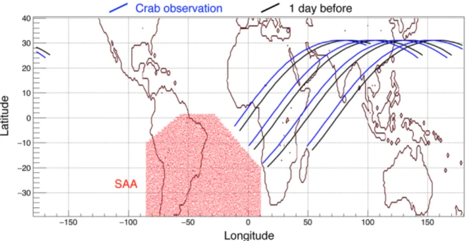
Fig. 1.Satellite position during observations. The black line shows the satellite position during the Crab GTI, and the blue line shows the position during the epoch one day earlier.

The attitude of the Hitomi satellite was stable throughout the Crab GTI. The nominal pointing position was (RA, Dec)=(83.^◦6334, 22.^◦0132) and the nominal roll angle was 267.^◦72, measured from the north to the satellite Y-axis counter-clockwise. The distance from the nominal pointing position was within 0.3 for 98.7% of the observa- tion time. The difference from the nominal roll angle was within 0.^◦05 for 99.6% of the observation time. Therefore, these offsets from the true direction of Crab are negligible and we have not considered them in the analysis.

2.2 Background determination

Figure1shows the Hitomi satellite position during the Crab GTI and one day before the Crab GTI, when the satellite was pointing at RXJ 1856.5−3754, which is a very weak source in the hard X-ray/soft gamma-ray band; such a “one day earlier” observation is thus a good proxy to measure the background. The time interval information for obser- vations performed one day earlier than the Crab GTI are listed in table3. Because the observations started soon after the SAA passages, the background rate during the Crab

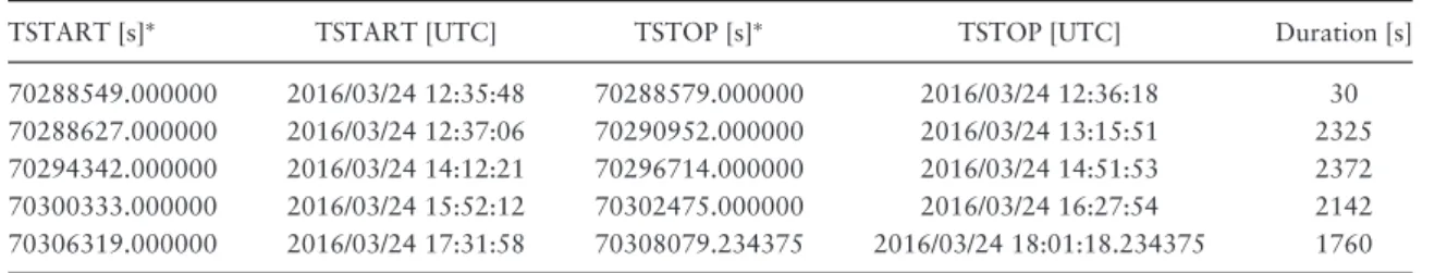
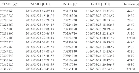
Table 3.Time intervals of pointings performed one day earlier than the Crab GTI.

TSTART [s]^∗ TSTART [UTC] TSTOP [s]^∗ TSTOP [UTC] Duration [s]

70288549.000000 2016/03/24 12:35:48 70288579.000000 2016/03/24 12:36:18 30 70288627.000000 2016/03/24 12:37:06 70290952.000000 2016/03/24 13:15:51 2325 70294342.000000 2016/03/24 14:12:21 70296714.000000 2016/03/24 14:51:53 2372 70300333.000000 2016/03/24 15:52:12 70302475.000000 2016/03/24 16:27:54 2142 70306319.000000 2016/03/24 17:31:58 70308079.234375 2016/03/24 18:01:18.234375 1760

∗TSTART and TSTOP are expressed in AHTIME, defined as the time elapsed since 2014/01/01 00:00:00 in seconds.

Fig. 2.Spectra of CdTe side single-hit events. The red and black points show the spectra for one day and two days earlier than the Crab GTI, respectively. The blue spectrum shows the single-hit events of the CdTe side sensors on an orbit when the satellite did not pass the SAA region.

GTI was higher than the average due to short-lived acti- vated materials produced in the SAA. Although the Crab nebula is one of the brightest sources in this energy region, the background events were not negligible for spectral anal- ysis and polarization measurements. As shown in figure1, the satellite positions and orbit conditions one day earlier than the Crab GTI were similar to those during the Crab GTI, which would imply background conditions could be similar.

In order to confirm that the satellite encountered sim- ilar background environments during similar orbit condi- tions, we compare the SGD data between an epoch one day earlier and also two days earlier than the Crab obser- vation GTIs. The single-hit spectra obtained by the CdTe side sensors are shown in figure2. The CdTe side sensors are located on the four sides around the stack of Si/CdTe sensors inside the Compton camera, and are not exposed to gamma-rays from the field of view. Therefore, the influence of the background environment should be reflected strongly in the single-hit events in the CdTe side detectors. The red

Fig. 3.Count rate of the SGD Compton camera as a function of time. The red and blue points show the count rates during the Crab observation and one day earlier. The black points show the count rates of the Crab GTI after subtracting the count rates one day earlier. The regions filled in green show the Crab GTI. The regions filled in cyan show time intervals excluded from the GTI due to the SAA passages. In the“white”portions of the time intervals, the Crab nebula was not able to be observed because of Earth occultation.

and black points show the spectra for the epochs one day and two days earlier than the Crab GTI, respectively. These two spectra have the same spectral shape, including var- ious emission lines from activated materials. The flux levels were the same within 3%. On the other hand, the blue spec- trum shows the single-hit events of CdTe side detectors on an orbit where the satellite did not pass the SAA region.

Although the background environment varied during one day, it was found that background estimation becomes pos- sible by using the data from one day earlier.

In order to further verify the background subtraction using the data from one day earlier, the count rates as a function of time during the Crab GTI and one day earlier are compared in figure 3. The red and blue points show the count rates during the Crab GTI and one day earlier.

The black points show the count rates of the Crab GTI after subtracting the count rates one day earlier, which corresponds to the count rates of the Crab nebula. Since the black points do not show any visible systematic trend implying additional backgrounds, it implies that this back- ground subtraction is appropriate.

3 Data analysis

3.1 Data processing with Hitomi tools

The data processing and event reconstruction were per- formed by the standard Hitomi pipeline using the Hitomi ftools (Angelini et al. 2018).¹ In the pipeline process for SGD, the ftools used for the SGD were hxisgdsff, which converts the raw event data into the predefined data format,hxisgdpha, which calibrates the event energy, andsgdevtid, which reconstructs each event. These tools were included in HEASoft after version 6.19. The ver- sion of the calibration files used in this processing was 20140101v003.

One of key tools for SGD event reconstruction is sgdevtid, which determines whether the sequence of inter- actions is valid and computes the event energy and the three- dimensional coordinates of its first interaction. The event reconstruction procedure ofsgdevtidis described by Ichi- nohe et al. (2016). The first step of the process is to merge signals that are consistent with fluorescence X-rays with the original interaction sites according to their locations and energies. The merging process combines the separated signals into a hit for each interaction. The second step is to analyze the reconstructed hits and determine whether the sequence is consistent with an event. This step depends on the number of reconstructed hits. If there is only one hit, the process is performed, and the energy information and the hit position information are recorded in the output event file as a “single-hit” event. In the case of an event that has two to four hits, the process determines whether the event is a valid gamma-ray event and whether the first interaction is Compton scattering by applying the Compton kinematics equation:

cosθK=1−mec²

1

(E_γ−E1)− 1 E_γ

, (1)

whereθK is the scattering angle defined by Compton kine- matics, mec² is the rest energy of an electron, E1 is the first hit energy corresponding to the recoil energy of the scattered electron, and E_γ is the reconstructed energy of the incoming gamma-ray photon. All possible permuta- tions for the sequence of hits are tried and all sequences with non-physical Compton scattering angle (|cosθK| >

1) are rejected. Besides the kinematic scattering angle θK, the geometrical scattering angles θgeometry can be derived from the directions of the incident gamma-ray and the scat- tered gamma-ray. The incident gamma-ray is assumed to be aligned with the line of sight. The direction of the scat- tered gamma-ray is reconstructed from the positions of the

1https://heasarc.gsfc.nasa.gov/lheasoft/ftools/headas/hitomi.html.

first and second hits. Their difference is called the angular resolution measure (ARM):

ARM :=θK−θgeometry. (2)

If more than one sequence remains, the order of hits with the smallest ARM value is selected as the most likely sequence. Moreover, in the case of three-hit events, the second interaction is assumed to be Compton scattering, and, in the case of four-hit events, the second and third interactions are assumed to be Compton scatterings. For these interactions, the tests of Compton kinematics and dif- ferences between kinematic scattering angles and geomet- rical scattering angles are performed. If the sequences have any non-physical Compton scatterings or any kinematic angles inconsistent with the geometric scattering angles, the sequences are rejected. In the first calculation, the recon- structed energy of the incoming gamma-ray photonE_γ is set to be

E_γ =

i

Ei, (3)

where Ei is the energy information of the ith hit. For three-hit and four-hit events, if all sequences are rejected in this calculation,sgdevtidcalculates the escape energy, the unabsorbed part of the energy of a photon that is able to exit the camera after detections, and executes the previous tests again. Finally, for a good “Compton event” after the processing, the information for the first interaction such as cosθK, the azimuthal angleφ of scat- tered gamma-rays, and the ARM value as “OFFAXIS”

are recorded in the output event file in addition to the reconstructed energy information and the first-hit position information.²

3.2 Processing of Crab observation data

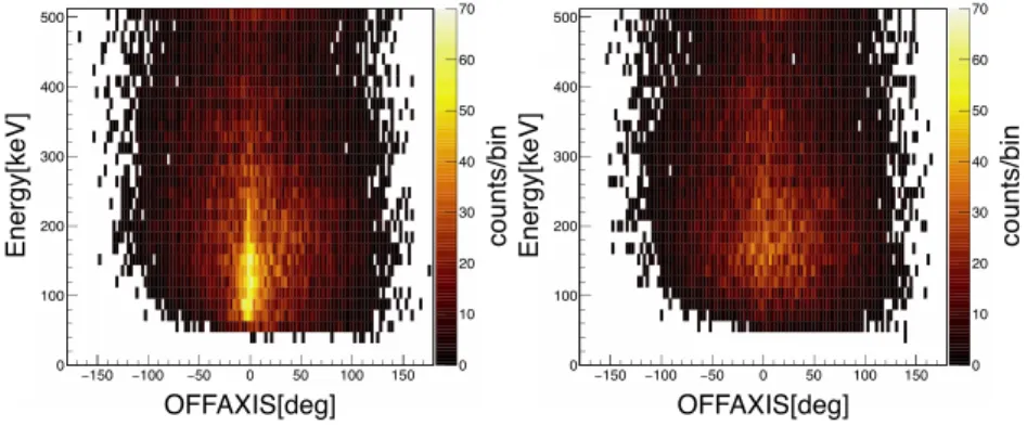
Figure4shows the relation betweenOFFAXIS and energy spectrum for the “Compton-reconstructed” events where sgdevtidfound the position of the first Compton scattering with physical cosθKin the Si sensors. The histogram in the left-hand panel is made from the events during the Crab GTI, and that in the right-hand panel is made from the events collected one day earlier than the Crab GTI. An excess at aroundOFFAXIS∼0^◦can be seen in the histogram of the Crab GTI corresponding to the gamma-rays from the Crab nebula.

In order to obtain a good signal-to-noise ratio, selections of 60 keV<Energy<160 keV,−30^◦ <OFFAXIS<+30^◦, 50^◦ < θgeometry < 150^◦ were applied. The histograms of

2The details of the columns recorded are shown athttps://heasarc.gsfc.nasa.gov/

ftools/caldb/help/sgdevtid.html.

Fig. 4.Two-dimensional histograms of Compton-reconstructed events. The relation betweenOFFAXISand energy is shown. The left-hand panel is the histogram made from the events during the Crab GTI; the right-hand panel is prepared from the events collected one day earlier than the Crab GTI.

Fig. 5.Histograms of Energy,OFFAXIS,θgeometry. The selection criteria were 60 keV<Energy<160 keV,−30^◦<OFFAXIS<+30^◦, and 50^◦< θgeometry

<150^◦. The red histograms are made from the events during the Crab GTI, and the black ones are from the events during the epoch one day earlier than the Crab GTI.

Energy, OFFAXIS, and θgeometry are shown in figure5. The selections of Energy,OFFAXIS, andθgeometrywere not applied in the histograms of Energy,OFFAXIS, andθgeometry, respec- tively. The red histograms are made from the events during the Crab GTI, and the events collected during the period one day earlier than the Crab GTI are shown in black as a reference.

We measured the gamma-ray polarization by inves- tigating the azimuth angle distribution in the Compton camera, since gamma-rays tend to be scattered perpendic- ular to the direction of the polarization vector of the inci- dent gamma-ray in Compton scatterings. Figure 6shows the azimuth angle distribution of Compton events obtained with the SGD Compton cameras. The red and the black points show the distribution during the Crab GTI and that from one day earlier than the Crab GTI, respectively. The azimuthal angleis defined as the angle from the satellite +X-axis to the satellite +Y-axis. The average count rate during the Crab GTI was 0.808 count s⁻¹.

Fig. 6.Azimuth angle distributions obtained with the SGD Compton cameras. The red and black points show the distribution during the Crab GTI and that from an epoch one day earlier than the Crab GTI, respectively. The definition ofis also shown. SATX and SATY mean the satellite+X-axis and the satellite+Y-axis, respectively.

Table 4.Good time intervals of the RXJ 1856.5−3754 observation.

TSTART [s]^∗ TSTART [UTC] TSTOP [s]^∗ TSTOP [UTC] Duration [s]

70207640 2016/03/23 14:07:19 70212120 2016/03/23 15:21:59 4480 70213720 2016/03/23 15:48:39 70218300 2016/03/23 17:04:59 4580 70219740 2016/03/23 17:28:59 70221820 2016/03/23 18:03:39 2080 70221860 2016/03/23 18:04:19 70224420 2016/03/23 18:46:59 2560 70225700 2016/03/23 19:08:19 70230580 2016/03/23 20:29:39 4880 70231600 2016/03/23 20:46:39 70236720 2016/03/23 22:11:59 5120 70237100 2016/03/23 22:18:19 70274520 2016/03/24 08:41:59 37420 70275720 2016/03/24 09:01:59 70280400 2016/03/24 10:19:59 4680 70287960 2016/03/24 12:25:59 70292460 2016/03/24 13:40:59 4500 70294120 2016/03/24 14:08:39 70298640 2016/03/24 15:23:59 4520 70300140 2016/03/24 15:48:59 70304760 2016/03/24 17:05:59 4620 70306140 2016/03/24 17:28:59 70310880 2016/03/24 18:47:59 4740 70312120 2016/03/24 19:08:39 70317050 2016/03/24 20:30:49 4930 70317950 2016/03/24 20:45:49 70355100 2016/03/25 07:04:59 37150

∗The unit for TSTART and TSTOP is AHTIME.

Table 5.Exposures of the RXJ 1856.5−3754 observation.

Live time

SGD1 CC1 84358.5

SGD1 CC2 84432.5

SGD1 CC3 84559.5

SGD2 CC1 89159.2

3.3 Background estimation for polarization analysis

Before the Crab observations, Hitomi also observed RXJ 1856.5−3754, which is fairly faint in the energy band of the SGD (Hitomi Soft X-ray Imager results were reported in Nakajima et al. 2018). The GTIs of RXJ 1856.5−3754 and the exposure times are listed in tables4 and 5, respectively. The total exposure time of the RXJ 1856.5−3754 observation was about 85.6 ks, and the number of Compton-reconstructed events about 24400.

More than ten times the number of events are available by using this observation than the observation of the Crab nebula. In order to obtain the azimuth angle dis- tribution of the background events with better statistics, the SGD data during the RXJ 1856.5−3754 GTI were investigated.

Comparisons of the incident energy,OFFAXIS,θgeometry, and the azimuth anglebetween the RXJ 1856.5−3754 GTI and one day earlier than the Crab GTI are shown in figure7. Since orbits with no SAA passage are included in the RXJ 1856.5−3754 observation, the flux level was lower than that obtained one day earlier than the Crab GTI. The count rate of the events during the RXJ 1856.5−3754 GTI

was 0.285 count s⁻¹, and that one day earlier than the Crab GTI was 0.404 count s⁻¹. Therefore, the scale of the his- tograms for the RXJ 1856.5−3754 GTI are normalized to match those for one day earlier than the Crab GTI. The distributions of OFFAXIS,θgeometry, and the azimuth angle are similar. Since the incident energy spectrum of the RXJ 1856.5−3754 GTI looks slightly different from that observed one day earlier than the Crab GTI, we further investigated the effect on thedistribution. We divided the data into five energy bands, 60–80 keV, 80–100 keV, 100–

120 keV, 120–140 keV, and 140–160 keV, and the number of events in each energy band was normalized to match those for one day earlier than the Crab GTI. The resulting distribution for the RXJ 1856.5−3754 GTI is shown as the magenta points in the lower-right panel of figure7. We do not observe any significant trend from the original distri- bution for the RXJ 1856.5−3754 GTI, which implies that the difference in the energy spectrum does not have a sig- nificant effect on thedistribution. From the above inves- tigations, we conclude that the Compton-reconstructed events during the RXJ 1856.5−3754 GTI can be uti- lized for the background estimation of the polarization analysis.

3.4 Monte Carlo simulation

Monte Carlo simulations of SGD are essential to derive the physical parameters, including the gamma-ray polar- ization, from the observation data. For the Monte Carlo simulations, we used ComptonSoft³in combination with a mass model of the SGD and databases describing detector

3https://github.com/odakahirokazu/ComptonSoft.

Fig. 7.Comparisons between the RXJ 1856.5−3754 observation and those obtained one day earlier than the Crab GTI. The green and black points show the RXJ 1856.5−3754 observation data and the data from one day earlier than the Crab GTI, respectively. The black data points are identical to the black points in figures5and6. The normalizations of the histograms for the RXJ 1856.5−3754 observation are scaled to match the count rate of the one day earlier Crab GTI.

parameters that affect the detector response to polar- ized gamma rays. ComptonSoft is a general-purpose sim- ulation and analysis software suite for semiconductor radiation detectors including Compton cameras (Odaka et al. 2010), and depends on the GEANT4 toolkit library (Agostinelli et al.2003; Allison et al.2006,2016) for the Monte Carlo simulation of gamma-rays and their associ- ated particles. We chose GEANT4 version 10.03.p03 and G4EmLivermorePolarizedPhysicsas the physics model of electromagnetic processes. The mass model describes the entire structure of one SGD unit, including the surrounding BGO shields. The databases of the detector parameters con- tain configuration of readout electrodes, charge collection efficiencies, energy resolutions, trigger properties, and data readout thresholds in order to obtain accurate detector responses of the semiconductor detectors and scintillators composing the SGD unit.

The format of the simulation output file is same as the SGD observation data. The simulation data can be pro- cessed with sgdevtid and, as a result, it is guaranteed that the same event reconstructions are performed for both observation data and simulation data.

For the Compton camera part, the accuracy of the simu- lation response to the gamma-ray photons and the gamma- ray polarization was confirmed through polarized gamma- ray beam experiments performed at SPring-8 (Katsuta et al.

2016). The better than 3% systematic uncertainty was val- idated in the polarized gamma-ray beam experiments. On the other hand, the effective area losses due to the distor- tions and misalignments of the fine collimators (FCs) are not implemented in the SGD simulator (Tajima et al.2018).

We have not obtained measurements of the FC distortions and misalignments with the calibration observations: this is because the satellite operation was terminated before

Fig. 8.Single-hit spectra in the Si detectors of the Crab observation obtained with the four Compton cameras. The background-subtracted observation spectrum is shown in black, and the simulation spectrum is shown in cyan. In the simulation, a power-law spectrum,N·(E/1 keV)⁻ was assumed, with a photon index () of 2.1 andN=8.23.

we had the opportunity to make such measurements. In the simulator, ideal-shape FCs with no distortion and no misalignment are implemented. Since the losses due to the distortions and misalignments of the fine collimators do not affect the azimuthal angle distribution of the Compton scattering, the effects on the polarization measurements are negligible.

In the simulation of the Crab nebula emission we assumed a power-law spectrum, N · (E/1 keV)⁻, with a photon index () of 2.1. In the first step, unpolar- ized gamma-ray photons were assumed. Also, the nor- malization of the simulation model (N) was derived from the Si single-hit events. Figure 8 shows the Si single-hit spectrum obtained with the four Compton cameras. The background spectrum was estimated from the observations taken one day earlier than those for the Crab GTI, and the background-subtracted spectrum is shown in figure 8, together with the simulated spectrum. By scaling the inte- grated rate of the simulation spectrum in the 20–70 keV range to match the observed rate we obtained N=8.23, which corresponds to a flux of 1.89×10⁻⁸erg s⁻¹cm⁻²in the 2–10 keV energy range.

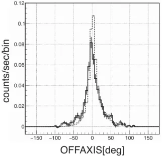
We compared the Compton-reconstructed events between the observation and the simulation. In figure9, the distributions ofOFFAXISfor the observation and the simu- lation are shown. The distribution ofOFFAXISfor the sim- ulation is slightly narrower than that for the observation.

If the same selection of−30^◦<OFFAXIS<+30^◦is applied

Fig. 9.Comparisons of the distributions ofOFFAXISevents between the observation and the simulation. The solid line and the dotted line show the observation data and the simulation data, respectively.

Fig. 10.Relation between the count rate and theOFFAXISselection for the simulation events. The count rate of 0.40 count s⁻¹derived from the observation data corresponds to theOFFAXISselection of 22.^◦13.

for both events, the observation count rate becomes 8.6%

smaller than the simulation count rate. We think that one cause of this discrepancy is in the modeling of the Doppler broadening profile of Compton scattering for electrons in silicon crystals. However, at this time, we have not found a solution to eliminate the discrepancy from first princi- ples. Therefore, by adjusting the OFFAXIS selection value of the simulation, we decided to match the count rate of the simulation to the observed count rate of 0.40 count s⁻¹. The relation between the count rate and theOFFAXISselec- tion for the simulation events is shown in figure10. From

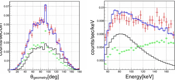
Fig. 11.Distribution ofθgeometry(left) and the energy spectrum (right). The observational data are plotted in red. The simulation data with the selection of−22.^◦13<OFFAXIS<+22.^◦13 are shown in black, and, the background data derived from the RXJ 1856.5−3754 observation are shown in green.

The sum of the simulation data and the background data is plotted in blue. The red data points are identical to the red ones in figure5, and the green data points are identical to the green ones in figure7.

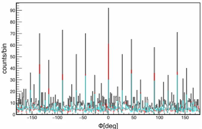
Fig. 12.Azimuth angle distributions of simulation data. Left: The azimuth angle distributions of the simulation data with theOFFAXISselection of

−22.^◦13<OFFAXIS<+22.^◦13 and−30^◦<OFFAXIS<+30^◦are shown in the solid line and the dotted line, respectively. The normalization for the

−30^◦<OFFAXIS<+30^◦selection is scaled. Right: The dependence of the azimuth angle distribution on the selectedOFFAXISvalue. This is shown as the ratio to theOFFAXISselection of three values to that limited to−22.^◦13<OFFAXIS<+22.^◦13. The black, red, and blue points show the results for OFFAXISselections of−30^◦<OFFAXIS<+30^◦,−15^◦<OFFAXIS<+15^◦, and−45^◦<OFFAXIS<+45^◦, respectively.

the relation, we obtained 22.^◦13 as the OFFAXIS selec- tion value of the simulation. The effect of adjusting the OFFAXISselection for the simulation is discussed later in this section.

The observational data, the background data, and the simulation data are plotted in figure 11. The simulation data with the selection of−22.^◦13<OFFAXIS<+22.^◦13 is shown in black, and the background data derived from the entire RXJ 1856.5−3754 observation is shown in green. The sum of the simulation data and the back- ground data is plotted in blue, and is comparable with the observation data shown in red. The θgeometry distri- bution is reproduced well by the Monte Carlo simu-

lation, while the energy spectrum shows a small dis- crepancy due to the background data, as shown in subsection 3.3.

The azimuth angle distributions of the simulated data are shown in figure 12. The left-hand panel shows the azimuth angle distributions of the simulated data with the OFFAXIS selection of −22.^◦13 <OFFAXIS <+22.^◦13 and

−30^◦ <OFFAXIS<+30^◦. The normalization for the−30^◦

<OFFAXIS<+30^◦selection is scaled. There is little differ- ence in the azimuth angle distribution between these two selections. The right-hand panel of figure12shows how the azimuth angle distribution depends on theOFFAXISselec- tion. It is found that the azimuth angle distribution changes