On a Coupled SPH-Rigid Body Method for the Surfing Problem

On a Coupled SPH‑Rigid Body Method for the Surfing Problem

著者 レザ レンディアン セプティアワン

著者別表示 Reza Rendian Septiawan journal or

publication title

博士論文本文Full 学位授与番号 13301甲第4816号

学位名 博士（理学）

学位授与年月日 2018‑09‑26

URL http://hdl.handle.net/2297/00053030

Creative Commons : 表示 ‑ 非営利 ‑ 改変禁止 http://creativecommons.org/licenses/by‑nc‑nd/3.0/deed.ja

Dissertation

On a Coupled SPH-Rigid Body Method for the Surfing Problem

Graduate School of

Natural Science and Technology Kanazawa University

Division of Mathematical and Physical Science

Student ID No. : 1524012017

Name : Reza Rendian Septiawan

Chief Advisor : Prof. Seiro Omata

Date of Submission : 29 June 2018

KANAZAWA UNIVERSITY

Abstract

Division of Mathematical and Physical Science Graduate School of Natural Science and Technology

PhD

On a Coupled SPH-Rigid Body Method for the Surfing Problem

by Reza Rendian Septiawan

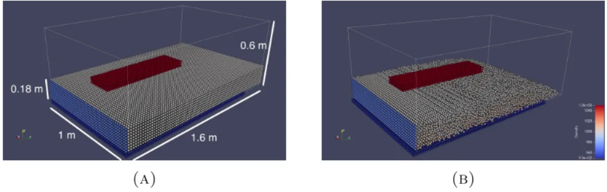
In this work, we use the smoothed particle hydrodynamics (SPH) method coupled

with a rigid body simulation to study the surfing problem. We simulate a surfing

board on top of an ocean wave which moves at a constant velocity. A fluid-rigid

body coupling is handled by using pure hydrodynamics-based force. External

forces are applied to the board, representing a surfer trying to stabilize the board

at a desired point along the uphill part of the ocean wave. An ordinary differential

equation (ODE) control is used to manipulate the distribution of the external

forces based on a position, velocity, and an inclination angle of the surfing board

relative to the ocean wave. The control system successfully helps the surfing board

to move and maintain its position at the desired point.

“So which of the favours of your Lord would you deny?”

(Quran 55:13)

Acknowledgements

First, the author would like to thank his Lord, Allah, for all of His blessings and favors.

The author would like to also thank all of his family members, for all of their love, support, and understanding. They help the author maintains his sanity all of the time.

The author would like to thank his Ph.D supervisor Professor Seiro Omata and Doctor Norbert Pozar for their invaluable supports, advices, and moral supports.

This work cannot be done without their help.

Next, the author would also like to thank to all of his friends, in campus and also outside campus, for all of their support, in academic life and also regular daily life.

The author would like to thank to Ministry of Education, Culture, Sports, Science, and Technology (MEXT) Japan for their financial support through MEXT U2U Scholarship.

iii

Contents

Abstract i

Acknowledgements iii

Contents iv

List of Figures vi

List of Tables vii

1 Introduction 1

1.1 Problem Statement . . . . 4

1.2 Goals . . . . 5

1.3 Outline of Dissertation . . . . 5

2 Governing Equations 7

2.1 Fluid Motion . . . . 7

2.1.1 Substantial Derivative . . . . 7

2.1.2 Transport Theorem . . . . 8

2.1.3 Conservation of Mass . . . 11

2.1.4 Conservation of Momentum . . . 12

2.1.5 Conservation of Energy . . . 17

2.2 Rigid Body Dynamics . . . 22

2.3 Linear analysis of the ODE control . . . 26

3 Smoothed Particle Hydrodynamics 31

3.1 Basic Idea of the SPH Method . . . 31

3.2 SPH Approximation for Fluid Dynamics . . . 33

3.3 Rigid Body Dynamics . . . 38

3.4 Rigid body discretization and coupling with SPH . . . 40

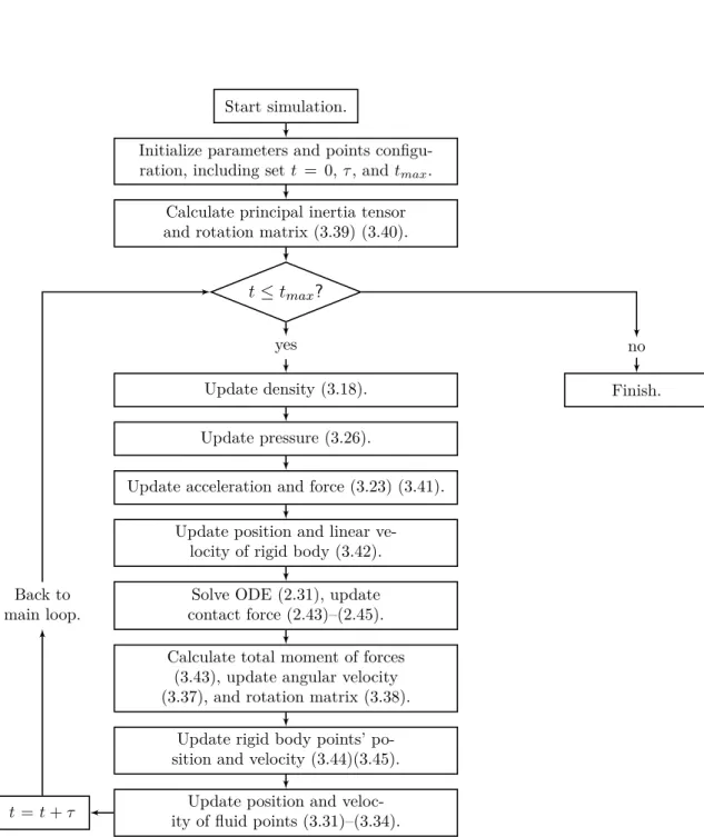
3.5 Algorithm of the simulation . . . 42

4 Results and Discussions 44

iv

Contents v 4.1 Set-up of the Simulation . . . 44 4.2 Results and Discussions . . . 46

5 Conclusion 51

5.1 Conclusions of The Work . . . 51 5.2 Future Work . . . 52

Bibliography 53

List of Figures

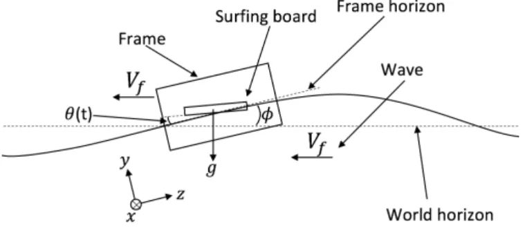
2.1 The illustration of the frame of system’s domain. . . 27

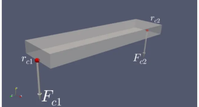
2.2 The locations of contact points. . . 30

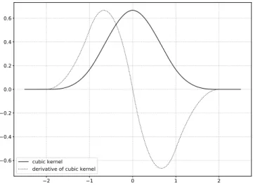
3.1 The graph of cubic kernel and its first derivative in 1D. . . 32

3.2 Algorithm of the simulation. . . 43

4.1 (a) The initial configuration of the system, and (b) the initial con- dition after relaxation process. . . 45

4.2 (A) The curve of positions in z-axis and inclination angles of the board through time without an ODE controller; snapshots of the surfing board simulation without an ODE controller at (B) t = 1.00 s, (C) t = 2.00 s, (D) t = 2.50 s, (E) t = 2.75 s. . . 46

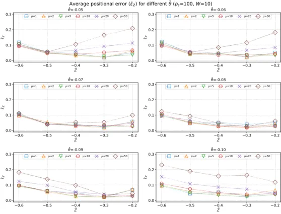
4.3 The graphs of the average positional error for different parameters θ, ˜ µ, and Z. . . 47 ˜

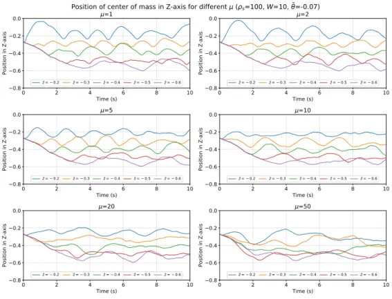
4.4 The z-axis-component position of surfing board for θ ˜ =

0.07. . . . 48

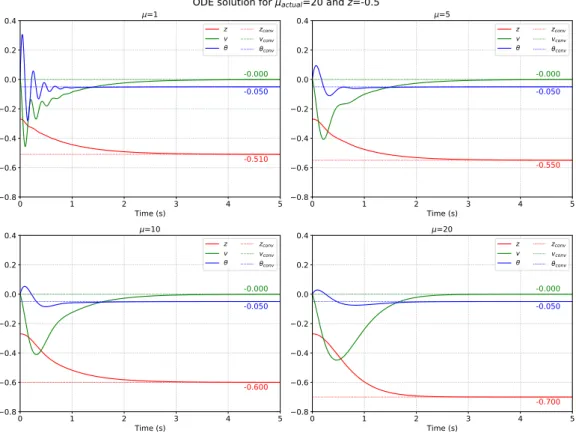
4.5 Solution of the ODE system for different µ. . . 49

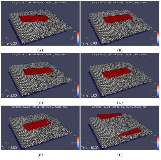
4.6 Snapshots of the surfing board simulation with an ODE controller with parameters Z ˜ =

0.2, µ = 5, and θ ˜ =

0.07 at (a) t = 0.20 s, (b) t = 0.90 s, (c) t = 2.50 s, (d) t = 5.00 s, (e) t = 8.00 s, and (f) t = 10.00 s. . . 50

vi

List of Tables

4.1 Table of the average of average positional error and its cumulative errors for each θ ˜ and µ. . . 47

vii

Dedicated to my beloved Mom and Dad. And for my whole family and friends for their love and support and

understanding. Because family and friends are always on the top priority.

viii

Chapter 1 Introduction

Surfing on ocean waves poses some interesting mathematical and physics problems.

One of them is a modeling of a surfer that controls the movement of the surfing board. The goal of what we called the surfing problem is to maintain the position of the surfing board on the upslope part of the ocean wave as long as possible. To reach the goal, the surfer maneuvers the surfing board by adjusting the distribution of forces given to the board via their feet in an attempt to modify the inclination angle of the surfing board.

To study the surfing problem, we can limit our domain frame to a small area of the uphill part of the ocean wave. This frame moves together with the wave, assuming the ocean wave moves with a constant velocity. In this dissertation we are developing an ordinary differential equation (ODE) control of the inclination angle of the surfing board to move the surfing board toward the desired point with respect to the wave. The ODE control that we propose is taking in the account of the position, velocity and the inclination angle of the surfing board.

The output inclination angle from the ODE control acts as a “target angle” for the surfing board. To reach the target angle we mimic the surfer’s attempt to control the board by giving two forces at the tips of the board. To find suitable parameters for which the control system is stable, we perform a stability analysis of a linearized simplified one-dimensional ODE model of the surfer on an ocean wave.

To verify the capabilities of the ODE control in controlling the movement of the rigid body under interaction with the fluid, we simulate the full system using the smoothed particle hydrodynamics (SPH) method. SPH is one of the most popular

1

Chapter 1. Introduction 2 Lagrangian solvers of the fluid equations. It was introduced by Lucy [1], and Gingold and Monaghan [2]. SPH method treats a system as a set of material points. Each material point brings physical informations and interacts with each others. In one of the original papers of SPH, Gingold and Monaghan [2] said that to recover the density from the known distribution of points, they need to recover a probability distribution from a sample, provided that the points are randomly distributed by their assumption. Because of its close relation with statistical ideas, therefore they described SPH as one of the Monte-Carlo methods. Later, in their next paper [3], they discussed that the motion of points is not sufficiently complex, therefore, the points cannot be considered as randomly distributed points through the whole domain.

Even though the SPH method is invented to approximate the numerical solution for the equations of fluid dynamics, at first the SPH method is developed to solve astronomical problems, such as a binary fission [1][3][4]. They modeled the motion of astronomical objects by the fluid dynamics equations with a dissipation term designed to stabilize the model before the system undergo the fission sequence.

Since then, the SPH method has been widely used in solving fluid dynamics prob- lems, such as shock wave problems. In [5], Gingold and Monaghan introduced a dissipative term designed to work with the SPH method since an artificial vis- cosity for finite difference scheme introduced in [6] produces excessive oscillation and smearing of the shock front due to the scale separation of points. Later they improved the artificial viscosity term to work with a subsonic flow [7]. Further, they use the solution from the Riemann problem to improve the artificial viscosity term for the SPH method in [8].

Another interesting fluid dynamics problems that can be solved by using the SPH

method are heat transfer problems. In [9] they successfully designed the heat

transfer model for the SPH method that can handle various problems of a heat

conduction, such as the heat conduction between points with different properties

(which implies points from different materials), a large discontinuity in a thermal

conductivity, a temperature-dependent thermal conductivity, and the most impor-

tant is the heat conduction with large deformation on material boundaries, which

is the main advantage of the SPH method compared to other methods such as

the finite difference method and the finite element method. Another heat transfer

problem which is interesting is the solidification process [10]. In that work they

improved the SPH method to deal with a phase-change phenomenon effectively,

Chapter 1. Introduction 3 starting from the Stefan problem associated with a fluid with a single composition, up to a fluid with multiple compositions, in their case, a sodium nitrate solution, and compared it with an experimental data. The result from the SPH method is in a good agreement with the experimental result.

Modeling the surface tension and the contact angle in a multi-phase simulation is also an interesting problem to be solved by using the SPH method. In [11] they proposed a combination of point-point interactions which incorporates a short- range repulsive interaction and a long-range attractive interaction to model a surface tension into the SPH method.

Numerous technical improvements to make the computation more efficient for the SPH method have been developed as well. One of them is by using a parallel computation. Parallelization in a numerical scheme is usually done by assigning different computation workers to solve the problem in fixed spatial subdomains while minimizing communication between workers, which is usually called a static load-balancing method. But since the SPH method is a Lagrangian solver, SPH points can move freely through the whole domain, causing non-uniform compu- tational load spatially, rendering a static load-balancing method inefficient. In [12], the dynamic load-balancing method for MPI protocol is used to improve the efficiency of parallel computing for the SPH method.

The computational capabilities of graphics processing unit (GPU) had a dramatic improvement in last several years, leads to a more common GPU utilization in many computational research fields, including fluid dynamics as well. Many trials have been done on implementing the SPH method into a GPU, but one of the difficulties comes from the neighbor searching algorithm which cannot be imple- mented in a trivial way on a GPU. One of the success studies of the SPH-GPU implementation is a massive parallelization with a GPU done in [13]. They suc- cesfully run the SPH simulation fully in a GPU, efficiently prevent a data transfer bottlenecking problem when one part of the simulation needs to be done on a CPU and the other part is run on a GPU.

Another interesting topic of research that can be solved by the SPH method is the

fluid-rigid body interaction. By the nature of the SPH method, boundary inter-

action between fluid and rigid body can be handled easily. Numerous studies on

an implementation of the SPH method to model the fluid-rigid body interaction

have been done by many researchers from different fields of study. One of the

Chapter 1. Introduction 4 studies related to the simulation of the fluid-rigid body interaction by using the SPH method is [14]. They studied the impact of a rigid body when it hits the body of water, by using both laboratory experiments and numerical simulations.

They modeled the interaction between the rigid body and the fluid by discretizing the rigid body into a set of boundary points that can interact with other SPH fluid points. The interaction between both types of points is done by exchang- ing momentum via a Lennard-Jones potential repulsive boundary force, which is called the Monaghan boundary force (MBF). The MBF is designed to prevent penetration of fluid points with a maximum velocity into a rigid body. However, the repulsive force from the MBF is thought to be too strong for a slow moving points. In [15] an impulse-based boundary force (IBF) was proposed. Recently, a more robust IBF is introduced in [16] by using a sequential impulse to solve the frictional contact problem with many contact points.

The IBF method relies heavily on the normal of the surface of rigid bodies. Hence, for a complex-shaped rigid body, the calculation is difficult. Moreover, IBF does not use pure hydrodynamics-based forces. A more versatile fluid-rigid body inter- action was introduced in [17]. By the inclusion of boundary points in the density calculation, they also solved a neighbor deficiency problem near the boundary which is a common problem in the SPH method.

1.1 Problem Statement

In this dissertation we want to study a surfing problem. In what we call a surfing problem, the goal is to maintain the surfing board to stay on top of the upslope part of the ocean wave as long as possible. In an attempt to achieve this goal, the surfer needs to control the movement of the surfing board by utilizing his/her own body weight, balancing the net force between the drag force and the gravity. Here we propose an ODE control that can help the surfing board maintains its position at a desired point on the uphill part of the ocean wave.

The author uses SPH as his method of choice to simulate the surfing problem since

the SPH method is capable to handle the free surface fluid motion. This problem

is interesting since it combines two things at once; modeling of the ocean wave

by a coupled fluid-rigid body simulation by using the SPH method and the ODE

control to help the surfing board maintains its position.

Chapter 1. Introduction 5 Simulating the ocean wave with the surfing board is one of the main challenges in this study, since there is a large scale difference between both the ocean wave and the board. By choosing a right frame of reference, we can take just enough part of the ocean that we need to study our case. Another main challenge here is in the process of designing the ODE control that could incorporate all parameters that affect the motion of the surfing board, while still make it simple enough to be analysed easily. The result of the work in this dissertation is published in [18].

1.2 Goals

The goals of this study are:

1. Propose an ODE control that can control and maintain the position of the surfing board at a given desired point.

2. Design a coupled fluid-rigid body simulation using the SPH method that can model the movement of surfing board on top of an ocean wave.

1.3 Outline of Dissertation

This dissertation consists of 5 chapters that are briefed as follows.

Chapter 1

tells a description of the surfing problem and a brief history about the development of the SPH method over years since its invention. In this chapter the author cites several articles which give fundamental impacts to the SPH method overall and also related to this dissertation. The author also writes the main problem and the objectives of this study. This chapter is ended by an outline of the whole dissertation.

Chapter 2

explains about equations govern the problem stated in this disser- tation. Starting from a set of governing equations for the hydrodynamics, then continued to the rigid body dynamics, and ended with a linear analysis of the ODE control.

Chapter 3

describes a fundamental theory of the SPH method. This chapter

provides an SPH approximation for fluid dynamics, the implementation of rigid

body simulation into SPH method, and the algorithm of the simulation.

Chapter 1. Introduction 6

presents the setup of the simulation and the results of the simulation.

In this chapter we will discuss about the results that we ge from the simulation as well.

Chapter 5

finally presents the conclusion of this work and a plan for the future

works which have not yet been achieved through this work.

Chapter 2

Governing Equations

2.1 Fluid Motion

2.1.1 Substantial Derivative

Let us have Ω

is a domain filled with a fluid at time t = 0. Next, consider that we have a material point of fluid is located at x

Ω

at time t = 0. The position of that material point at a given time t is X

(t), with X

(0) = x

, and its velocity is given by U

(t) =

X

(t). Since material points move, the shape of the domain changes with time. Let Ω

be the domain at a given time t. With a given x

Ω

, the velocity of a material point located at x = X

(t) at a given time t is defined as u(x, t) =

X

(t). u(x, t) for x

Ω

is so-called velocity field of the fluid.

All the above physical quantities notated using small alphabets are in an Eulerian description, which is fixed in space, while physical quantities notated with capital alphabets are in a Lagrangian description, with their information is moving with the material point. The relationship between velocity u in an Eulerian description with a material point velocity U from a Lagrangian description at a given time t can be written as U

(t) = u(X

(t), t). This relation also holds for other physical quantities that can be described in both descriptions, such as density.

To calculate the time derivative of a physical quantity F

(t) for a given material point x

(here, notation x

is also used to label the material point, which material point is located at x

Ω

at time t = 0), we need its ”counterpart” field function

7

Chapter 2. Governing Equations 8 f (x, t) in an Eulerian description. Let x = X

(t) = (X

(t), X

(t), X

(t))

Ω

for a given material point x

at time t, the velocity field is u(x, t) = u(X

(t), t) = u(X

(t), X

(t), X

(t), t) =

(X

(t), X

(t), X

(t)). The time derivative of F

(t) is

d

dt F

(t) = df

dt (X

(t), t)

= df

dt (X

(t), X

(t), X

(t), t)

= ∂f

∂t (X

(t), t) +

∑3 i=1

∂f

∂x

(X

(t), t) dX

(t) dt

= ∂f

∂t (X

(t), t) + u(X

(t), t)

f(X

(t), t)

=

∂f

∂t + u

f

(X

(t), t)

=: Df

Dt (X

(t), t).

The

D Dt = ∂

∂t + u

(2.1)

operator is called the substantial derivative (or sometimes, material derivative) operator.

2.1.2 Transport Theorem

Before we move to conservation laws, it is useful to introduce density functions for any measurable physical quantities, which means we can assign a value ψ(V

, t) to any given sufficiently nice subdomain V

Ω

at any given time t

[0,

), there exists a density function f = f(x, t) such that

ψ(V

, t) =

∫

Vt

f(x, t) dx .

Let us define a function ϕ(x

, t) := X

(t) as a function ϕ :

[0,

)

is smooth with a non-zero Jacobian matrix

D

ϕ(x

, t)

= 0,

x

, t

[0,

) so

1Capital D here represents a Jacobian matrix operator; neither related with substantial derivative nor with any physical units in a Lagrangian description.

Chapter 2. Governing Equations 9 the material points will not have an infinite density; and a function ϕ

(x

) :

defined as ϕ

(x

) := ϕ(x

, t) = X

(t) is invertible

t

[0,

) so that no more than one material point occupies the same position in space. A function ϕ is a flow map of the fluid which captures the kinematic evolution of the fluid. Above conditions guarantee that we have a nice regular flow, allow us to do the change of variables formula, differentiate, and integrate by parts.

Now let us consider a moving domain

V

which contains same material points for all time t, that is

X

(τ )

V

for some x

, τ

[0,

)

X

(t)

V

for all t

[0,

) , which implies

V

=

X

(t) : x

V

=

ϕ

(x

) : x

V

=: ϕ

(V

) .

Next let us introduce the Jacobian J(x

, t) to be the determinant of the Jacobian matrix of the function ϕ

at (x

),

J(x

, t) = det (Dϕ

(x

)) x

, t

[0,

) . (2.2)

Since material points cannot overlap with each others, the ”orientation” of the fluid remains the same and will not be flipped, hence, the Jacobian is non-negative. And since the Jacobian is also non-zero, so J (x

, t) = det(Dϕ

(x

)) > 0.

From the formula for the derivative of a determinant of an invertible matrix, d

dt det(A(t)) = det(A(t)) tr

A

(t) dA dt (t)

)

, we get

∂J

∂t (x

, t) = J(x

, t) tr

(Dϕ

(x

))

∂Dϕ

∂t (x

)

. (2.3)

Let us rewrite a velocity field u(x, t) in term of ϕ(x

, t) as u(ϕ(x

, t), t) = ∂ϕ

∂t (x

, t),

Chapter 2. Governing Equations 10 and differentiate the i-th component of both sides of the equation with respect to x

(let x

= (x

, x

, x

) and ϕ = (ϕ

, ϕ

, ϕ

)) as

∂u

∂x

(ϕ(x

, t), t) = ∂

∂t

∂ϕ

∂x

(x

, t)

∑

k

∂u

∂x

(ϕ(x

, t), t) ∂ϕ

∂x

(x

, t) = ∂

∂t

∂ϕ

∂x

(x

, t), which can be written as

D

u(ϕ(x

, t), t)Dϕ

(x

) = ∂

∂t Dϕ

(x

).

Since Dϕ

(x

) is invertible, we can multiply both sides of the equation by (Dϕ

(x

))

, take the trace, and use the property tr(AB) = tr(BA), we get

tr (D

u(ϕ(x

, t), t)) = tr

∂

∂t Dϕ

(x

)

(Dϕ

(x

))

= tr

(Dϕ

(x

))

∂

∂t Dϕ

(x

)

.

The left-hand side of the equation is tr (D

u(ϕ(x

, t), t)) = div(u(ϕ(x

, t), t)). Sub- stituting it back into equation (2.3) gives us

∂J

∂t (x

, t) = J(x

, t) div(u(ϕ(x

, t), t)). (2.4) Now we want to express the time derivative of ψ(V

, t) in terms of the derivative of its density function f. By the change of variables, we get

d dt

∫

Vt

f(x, t) dx = d dt

∫

V0

f (ϕ(x

, t), t) J(x

, t) dx

Since now the right-hand side is an integral over a domain which is independent of t, we can exchange integration and differentiation and we get

d dt

∫

Vt

f(x, t) dx =

∫

V0

∂

∂t (f(ϕ(x

, t), t) J (x

, t)) dx

. (2.5)

Chapter 2. Governing Equations 11 By the product rule, the chain rule, and substitution from (2.4), we have

∂

∂t (f (ϕ(x

, t), t) J(x

, t)) = f (ϕ(x

, t), t) ∂J

∂t (x

, t) + J(x

, t)

∂f

∂t + u

f

(ϕ(x

, t), t)

= f (ϕ(x

, t), t) (J(x

, t) div(u(ϕ(x, t), t))) + J (x

, t)

(

∂f

∂t + u

f

(ϕ

(x

, t), t)

= J (x

, t)

∂f

∂t + f div(u) + u

f

(ϕ(x

, t), t)

= J (x

, t)

∂f

∂t + div(f u)

(ϕ(x

, t), t)

. Finally, by substituting it back into (2.5) and by doing change of variables back into x and V

, we get

d dt

∫

Vt

f (x, t) dx =

∫

V0

(

∂f

∂t + div(f u)

(ϕ(x

, t), t)J (x

, t) dx

=

∫

Vt

(

∂f

∂t + div(f u)

(x, t) dx. (2.6)

Equation (2.6) is called The Transport Theorem.

2.1.3 Conservation of Mass

From continuum mechanics, we define density ρ in a given domain Ω

at a given time t as the function ρ

C(Ω), ρ :

[0,

)

s.t. m

(t) =

∫

Ω

ρ(x, t)dx, with m

(t) is a mass of fluid inside domain Ω at time t.

Let u be a velocity field and V be a fixed subdomain of Ω does not change with time. By using the conservation of mass, the rate of change of mass in V equals to total mass flow rate through the boundary of V (with normal vector n points outward),

d

dt m

(t) =

∫

∂V

ρ(x, t)u(x, t)

n(x, t) dS.

Chapter 2. Governing Equations 12 By using the divergence theorem for the right-hand side term, we get

d dt

∫

V

ρ(x, t) dx =

∫

V

div(ρ(x, t)u(x, t)) dx

∫

V

∂ρ(x, t)

∂t + div(ρ(x, t)u(x, t)) dx = 0. (2.7)

Since (2.7) must be true for any V

Ω,

∂ρ

∂t + div(ρu) = 0. (2.8)

Equation (2.8) is a continuity equation in an Eulerian description form.

By using a product rule for divergence, we get

∂ρ

∂t + div(ρu) = 0

∂ρ

∂t + ρ div(u) +

ρ

u = 0

∂ρ

∂t +

ρ =

ρ div(u) Dρ

Dt =

ρ div(u). (2.9)

Equation (2.9) is a continuity equation in a Lagrangian description form.

2.1.4 Conservation of Momentum

Forces acting on a material body can be classified into two types: stress forces act on the surface, and body (or external) forces act on the continuum itself.

The simplest type of stress forces is a pressure force, as stated from [19] pp 5, is defined as, for any motion of the fluid there is a function p(x, t) called the

such that if S is a surface in the fluid with a chosen unit normal n, the force of stress exerted across the surface S per unit area at x

S at time t is p(x, t)n; i.e.,

force across S per unit area =

p(x, t)n(x, t).

The pressure force is in the same direction with normal vector n, or in the other

words, orthogonal to the surface and does not have a tangential part.

Chapter 2. Governing Equations 13 Let S

be a total surface force acts on a given subdomain V

Ω at time t,

S

=

∫

∂V

p(x, t)n(x, t) dS,

where p is a pressure force, n is a normal vector points outward, and ∂V is a surface of V . By multiplying it with any fixed vector e

,

e

S

=

∫

∂V

p(x, t)e

n(x, t) dS

=

∫

V

div(p(x, t)e) dx

=

∫

V

p(x, t)div(e) + e

p(x, t) dx

=

∫

V

e

p(x, t) dx S

=

∫

V

∇

p(x, t) dx. (2.10)

Now let b be a given body force per unit mass. The total body force B

acts on V is

B

=

∫

V

ρ(x, t)b(x, t) dx. (2.11)

By definition, the linear momentum M(V, t) has a density function f(x, t) = ρ(x, t)u(x, t). Capital letter M here does not mean it is in a Lagrangian de- scription. By the Newton’s law, the rate of change of momentum equals to total force acts on the body. Using the similar argument with the conservation of mass, the rate of change of momentum equals to total momentum flow rate through the boundary plus rate of change of momentum by the source, which is in this case, total force acts on the body. Let M (V, t) = (M

(V, t), M

(V, t), M

(V, t)) and u(x, t) = (u

(x, t), u

(x, t), u

(x, t)), as well with S

= (S

, S

, S

), B

= (B

, B

, B

) and b = (b

, b

, b

). For i = 1, 2, 3 we have

d

dt M

(V, t) =

∫

∂V

ρ(x, t)u

(x, t)u

n dS + S

+ B

d dt

∫

V

ρ(x, t)u

(x, t) dx =

∫

V

div(ρ(x, t)u

(x, t)u(x, t)) dx

∫

V

∂

∂x

p(x, t) dx +

∫

V

ρ(x, t)b

(x, t) dx

Chapter 2. Governing Equations 14

∫

V

∂

∂t (ρ(x, t)u

(x, t)) dx =

∫

V

−

div(ρ(x, t)u

(x, t)u(x, t))

−

∂

∂x

p(x, t) + ρ(x, t)b

(x, t) dx.

Since all ρ, p, b, and u (and, of course, u

for i = 1, 2, 3) are functions of (x, t), let us drop it from the equation for simplicity. Since the equation must be true for any V

Ω, the equation becomes

∂(ρu

)

∂t + div(ρu

u) =

∂p

∂x

+ ρb

, (2.12)

which is an Eulerian description for conservation of momentum. By doing product rules, we get

−

∂p

∂x

+ ρb

= ρ ∂u

∂t + u

∂ρ

∂t + ρu

div(u) + ρu

div(u

) + u

u

div(ρ)

= ρ

∂u

∂t + u

div(u

)

+ u

∂ρ

∂t + ρdiv(u) + u

div(ρ)

= ρ Du

Dt + u

(

∂ρ

∂t + div(ρu)

.

By using (2.8), the second term of right-hand side of the equation became zero, leaving us with

ρ Du

Dt =

∂p

∂x

+ ρb

, or

ρ Du

Dt =

p + ρb, (2.13)

which is a Lagrangian description for the conservation of momentum.

As mentioned before, (2.12) and (2.13) assume that the only force exerts on the surface comes from the pressure term which is in an orthogonal direction to the surface, which is the case of an inviscid flow of the fluid. Next we will try to take into account a tangential part of the force as well. Let us modify our previous definition into

force across S per unit area =

p(x, t)n(x, t) + σ(x, t)

n(x, t),

with σ is a matrix called stress tensor, fulfills some assumptions:

Chapter 2. Governing Equations 15 1. σ depends linearly to

that is, the stress tensor σ is related to the gradient

of the velocity field

by some linear transfomations at each points.

2. σ is invariant under rigid body rotation, that is, let U is an orthogonal matrix,

σ(U

U

) = U

σ(Du)

U

. 3. σ is symmetric.

Du

consists of two parts, a symmetric part

=

(Du + (Du)

) which represents the expansion or contraction of the fluid, hence denoted by

for ”deformation”, and a skew-symmetric

=

(Du

(Du)

) represents the rotation of fluid. It is easily can be checked that

=

+

Since σ is a symmetric matrix, by properties 1 and 2, it can only depends on a symmetric part of

σ is a linear function of

σ and

commute, and assuming both of them are diagonalizable, σ and

can be simultaneously diagonalized. Thus, the eigenvalues of σ are linear functions of the eigenvalues of

The only linear function which fulfils all conditions is

σ

= λ(d

+ d

+ d

) + 2µd

, i = 1, 2, 3, (2.14) where σ

are the eigenvalues of σ, d

are the eigenvalues of

λ and µ are constants.

d

+ d

+ d

equals to div(u), and by transforming it back to usual basis, we get

σ = λ div(u)I + 2µD, (2.15)

where

is an identity matrix. By rearranging the equation, we get:

σ = 2µ

D−

1

3 div(u)I

+ ζ div(u)I, (2.16)

where µ is the first coefficient of viscosity and ζ = λ +

µ is the second coefficient

of viscosity.

Chapter 2. Governing Equations 16 Now the total surface force S

on a given subdomain V

Ω at a given time t is given by (drop all variables (x, t) for simplicity),

S

=

∫

∂V

−

pn + σ

n dS

=

∫

∂V

−

pn + (λ div(u)I + 2µD)

n dS

=

∫

∂V

pn dS + λ

∫

∂V

div(u)n dS + 2µ

∫

∂V

1

2 ((Du) + (Du)

) dS

=

∫

∂V

pn dS + λ

∫

∂V

div(u)n dS + µ

∫

∂V

((Du) + (Du)

) dS.

By multiplying it with a fixed vector e

we have e

S

=

∫

∂V

pe

n dS + λ

∫

∂V

div(u)e

n dS + µe

∫

∂V

(Du + (Du)

) dS

=

∫

V

div(pe) dx + λ

∫

V

div(div(u)e) dx + µe

∫

V

(div(Du) + div((Du)

)) dx.

Since e is fixed, the product rule of div(f e) = e

f for any scalar function f . Also,

(div((Du)

))

=

∑3 j=1

∂

∂x

((Du)

)

=

∑3 j=1

∂

∂x

(Du)

=

∑3 j=1

∂

∂x

∂u

∂x

= ∂

∂x

∑3 j=1

∂u

∂x

= (

(div(u)))

, or

div((Du)

) =

(div(u)).

Let us denote ∆u =

∂x²₁

+

+

3

)

u = div(Du) is a Laplacian of the velocity field u. Back to the total surface force, now we have

e

S

=

e

∫

V

∇

p dx + λe

∫

V

∇

(div(u)) dx + µe

∫

V

∆u +

(div(u)) dx

= e

∫

V

−∇

p + (λ + µ)

(div(u)) + µ∆u dx S

=

∫

V

−∇

p + (λ + µ)

(div(u)) + µ∆u dx.

Chapter 2. Governing Equations 17 By doing the similar things like before, by the conservation of momentum (and dropping all variables (x, t)), we have

d

dt M

=

∫

∂V

ρu

u

n dS + S

+ B

d

dt

∫

V

ρu

dx =

∫

V

div(ρu

u) dx +

∫

V

−

∂p

∂x

+ (λ + µ) ∂

∂x

(div(u)) + µ∆u

dx +

∫

V

ρb

dx

∫

V

∂

∂t (ρu

) dx =

∫

V

−

div(ρu

u)

∂p

∂x

+ (λ + µ) ∂

∂x

(div(u)) + µ∆u

+ ρb

dx.

Since it must be true for any V

Ω,

∂(ρu

)

∂t + div(ρu

u) =

∂p

∂x

+ (λ + µ) ∂

∂x

(div(u)) + µ∆u

+ ρb

. (2.17) (2.17) is an Eulerian description of conservation of momentum for viscous fluid.

We also have ρ Du

Dt =

∂p

∂x

+ (λ + µ) ∂

∂x

(div(u)) + µ∆u

+ ρb

, or

ρ Du

Dt =

p + (λ + µ)

(div(u)) + µ∆u + ρb, (2.18) which is a Lagrangian description of conservation of momentum for viscous fluid.

2.1.5 Conservation of Energy

The total energy E(V

, t) for the moving volume V

= V (t)

Ω at a given time t is the summation of its kinetic energy E

(V

, t) and the internal energy E

(V

, t).

The kinetic energy of V

is defined as E

(V

, t) = 1

2

∫

Vt

ρ(x, t)

u(x, t)

dx,

where ρ(x, t)

u(x, t)

is the density function of the kinetic energy, and

u(x, t)

=

u(x, t)

u(x, t) = u

(x, t) + u

(x, t) + u

(x, t). By using the transport theorem, the

Chapter 2. Governing Equations 18 rate of change of the kinetic energy is written as

d

dt E

(V

, t) = 1 2

d dt

∫

Vt

ρ(x, t)

u(x, t)

dx

= 1 2

∫

Vt

(

∂

∂t (ρ

u

) + div(ρ

u

u)

(x, t) dx

= 1 2

∫

Vt

(

ρ ∂

u

∂t +

u

∂ρ

∂t + ρ div(

u

u) +

u

u

ρ

(x, t) dx

= 1 2

∫

Vt

(

ρ ∂

u

∂t +

u

∂ρ

∂t + ρ

u

div(u) + ρu

(

u

) +

u

u

ρ

)

(x, t) dx

= 1 2

∫

Vt

(

∥

u

∂ρ

∂t + u

ρ + ρ div(u)

+ ρ

(

∂

u

∂t + u

∥

u

(x, t) dx.

By using the conservation of mass, the first term is zero, and for the second term we will substitute:

∂

u

∂t + u

(

u

) = ∂(u

u)

∂t + u

(u

u)

= 2u

∂u

∂t +

∑3 i=1

u

(

(u

u))

= 2u

∂u

∂t +

∑3 i=1

u

∂

∂x

( ₃

∑

j=1

u

u

= 2u

∂u

∂t + 2

∑3 i=1

∑3 j=1

u

u

∂u

∂x

= 2

u

∂u

∂t +

∑3 j=1

u

∑3 i=1

u

∂u

∂x

= 2

u

∂u

∂t + u

(u

)u

. So now we have

d

dt E

(V

, t) = 1 2

∫

Vt

(

ρ

(

∂

u

∂t + u

∥

u

(x, t) dx

=

∫

Vt

(

ρu

(

∂u

∂t + (u

)u

(x, t) dx, (2.19)

Chapter 2. Governing Equations 19 where

(u

)u =

∑

j=1

u

∂u

∂x

i=1...3

.

In general, we will do a similar thing like before for the conservation of energy.

The total time rate of change of the energy equals to the total heat flux into the system plus the total rate of works done by forces. Before we continue, we need to discuss about a case of an incompressible flow.

The incompressible fluid means that the volume of the fluid will not change with time. By the change of variables and (2.4), for a moving fluid element V

at a given time t, we have

d

dt

V

= d dt

∫

Vt

dx = d dt

∫

V0

J (x

, t) dx

=

∫

V0

∂J

∂t (x

, t) dx

=

∫

V0

div(u(ϕ(x

, t), t))J (x

, t) dx

=

∫

Vt

div(u(x, t)) dx = 0,

which implies that div(u) = 0 for any V

, with

V

is the measure of the volume V

. By assuming the kinetic energy is the only energy works on the system, and by the definition of works, for an inviscid incompressible fluid, the rate of change of the energy of V

at time t is

d

dt E

(V

, t) =

∫

∂Vt

(pu

n)(x, t) dS +

∫

Vt

(ρu

b)(x, t) dx

∫

Vt

(

ρu

(

∂u

∂t + (u

)u

(x, t) dx =

∫

V

(

div(pu) + ρu

b) (x, t) dx

=

∫

Vt

(

u

p + ρu

b) (x, t) dx, since div(u) = 0 for an incompressible case. So now we have

∫

Vt

(

u

(

ρ Du

Dt

(x, t) dx =

∫

Vt

(u

(

p + ρb)) (x, t) dx.

This equation is also a consequence of the balance of momentum. This shows that

if we only assume E = E

, then the fluid must be an incompressible fluid (except

if we have p = 0 for the whole domain).