On a Coupled SPH-Rigid Body Method for the Surfing Problem

(1)

Surfing Problem

著者レザレンディアンセプティアワン

著者別表示 Reza Rendian Septiawan journal or

publication title

博士論文要旨Abstract 学位授与番号 13301甲第4816号

学位名博士（理学）

学位授与年月日 2018‑09‑26

URL http://hdl.handle.net/2297/00053029

Creative Commons : 表示 ‑ 非営利 ‑ 改変禁止 http://creativecommons.org/licenses/by‑nc‑nd/3.0/deed.ja

(2)

Dissertation Abstract

On a Coupled SPH-Rigid Body Method for the Surfing Problem

Graduate School of

Natural Science and Technology Kanazawa University

Division of Mathematical and Physical Science

Student ID No. : 1524012017

Name : Reza Rendian Septiawan Chief Advisor : Prof. Seiro Omata

Date of Submission : 29 June 2018

(3)

In this work, we use the smoothed particle hydrodynamics (SPH) method coupled with a rigid body simulation to study the surfing problem. We simulate a surfing board on top of an ocean wave which moves at a constant velocity. A fluid-rigid body coupling is handled by using pure hydrodynamics-based force. External forces are applied to the board, representing a surfer trying to stabilize the board at a desired point along the uphill part of the ocean wave. An ordinary differential equation (ODE) control is used to manipulate the distribution of the external forces based on a position, velocity, and an inclination angle of the surfing board relative to the ocean wave. The control system successfully helps the surfing board to move and maintain its position at the desired point.

Dissertation Abstract

1 Introduction

In what we called the surfing problem, the goal is to maintain the position of the surfing board on top of the upslope part of the ocean wave as long as possible. In this work we propose an ODE control that is capable to control the movement of the surfing board and maintain the position of the surfing board to be at a given desired point. Here we validate the ODE control by performing a coupled fluid-rigid body SPH simulation for the surfing problem.

2 Governing Equations

2.1 Fluid Dynamics

The motion of fluid is governed by following conservation laws which are the Euler’s equations of the fluid dynamics [1]:

1. Conservation of mass:

Dρ

Dt =−ρdiv(u),

2. Conservation of momentum:

Du Dt =−1

ρ∇p+b,

whereρ, p, and uare density, pressure, and velocity field, respectively,b is a body force per unit mass, and

D

Dt is a so-called substantial derivativedefined as ^Df_Dt = ^∂f_∂t +u· ∇f for any field functionf(x, t), withuis a velocity field.

2.2 Rigid Body Dynamics

Rigid body can only undergo a linear and a rotational transformation which follow the conservation of a linear momentum and the conservation of an angular momentum, respectively.

1. Conservation of linear momentum:

dG(t)

dt =F(t),

2. Conservation of angular momentum:

dL(t)

dt =K(t),

where G(t) = M U(t) and L(t) = J(t)ω(t) are a linear momentum and an angular momentum of the rigid body at a given timet, respectively, withM,U,J, andωare a mass, linear velocity of the rigid body, moment of inertia tensor, and an angular velocity of the rigid body, respectively. We can choose such a reference configuration of the rigid body so we can have a moment of inertia tensor to be a diagonal matrixJˆ called a principal moment of inertia tensor. LetR(t)be an orthogonal rotation matrix of the rigid body at a given

(4)

(a)

0 1 2 3 4 5

Time (s) 0.8

0.6 0.4 0.2 0.0 0.2 0.4

-0.510 -0.000 -0.050

=1 zv zconv

vconv conv

0 1 2 3 4 5

Time (s) 0.8

0.6 0.4 0.2 0.0 0.2 0.4

-0.550 -0.000 -0.050

=5 zv zconv

vconv conv

0 1 2 3 4 5

Time (s) 0.8

0.6 0.4 0.2 0.0 0.2 0.4

-0.600 -0.000 -0.050

=10 zv zconv

vconv conv

0 1 2 3 4 5

Time (s) 0.8

0.6 0.4 0.2 0.0 0.2 0.4

-0.700 -0.000 -0.050

=20 zv zconv

vconv conv

ODE solution for actual=20 and z=-0.5

(b)

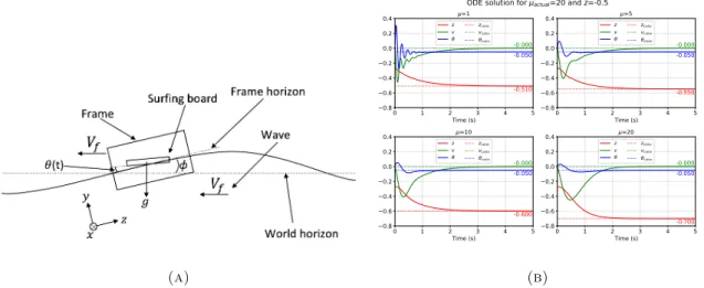
Figure 1: (A) Sideview of the illustration of the frame of system’s domain, (B) Solution of the ODE by using direct ODE solver.

timet. The angular velocity is defined as a vectorω(t) = (ω1(t), ω2(t), ω3(t))satisfies

d

dtR(t) =W(t)R(t), W(t) =







0 −ω3(t) ω2(t) ω3(t) 0 −ω1(t)

−ω₂(t) ω₁(t) 0





.

This leads to the Euler’s equation of the rigid body dynamics, ˆ

ω(t)×Jˆˆω(t) + ˆJω(t) = ˆ˙ˆ K(t),

whereK(t) =ˆ R^T(t)K(t),ω(t) =ˆ R^T(t)ω(t), andω(t) =˙ˆ ^d^ω(t)^ˆ_dt .

2.3 ODE Control

We choose the frame of the system to be parallel with the upslope part of the ocean wave and moves together with the ocean wave with a constant velocity (see Figure 1a).

The goal of the surfing problem is to control the position of the surfing board to be at the desired point.

Here we want to control the surfing board on one axis only, in this case, theZ-axis. The only parameter that we can control is the inclination angle of the surfing board. We propose the following ODE control for the inclination angle,

θ(t) =˙ a(Z(t)−Z˜) +b(V(t)−V˜) +c(θ(t)−θ),˜ (1)

whereZ and V are the third component of position and linear velocity of the surfing board, respectively,θ is the inclination angle of the surfing board,Z˜, V˜, and θ˜are the desired position, velocity, and the desired inclination angle, respectively. Because of the choice of the frame, we setV˜ = 0. Z˜ is given. Up to now we do not have any information aboutθ.˜ a, b, andc are given parameters that can make the system stable.

To find suitable parameters for a, b, and c, we consider a simplified linearized ODE model with the ODE control (1).









Z(t)˙ =V(t),

V˙(t) =−µθ(t)−µvV(t)−µzZ(t)−µ0, θ(t)˙ =a(Z(t)−Z) +˜ bV(t) +c(θ(t)−θ),˜

(2)

(5)

Figure 2: The locations of contact points.

whereµ,µv,µz, andµ0are constants related to the drag and gravity forces. For now let us assumeµv =µz= 0 for simplicity. Although the assumption is not correct, it does not seem to influence the stability of the system.

We can write (2) in a matrix form as

ξ(t) =˙







0 1 0

0 0 −µ

a b c





ξ(t) +





 0

−µ₀ 0





=:Aξ(t) +ζ.

The stationary point will be stable if all eigenvalues of matrixAhave negative real parts. The characteristic equation ofAis

det(A−λI) =−λ³+cλ²−bµλ−aµ= 0. (3)

Let us set the roots of (3) to beλ1=−3,λ2=−4, andλ3=−5. This yields the equation

−λ³−12λ²−47λ−60 = 0. (4)

Comparing (4) with (3), we geta= ⁶⁰_µ, b= ⁴⁷_µ, and c=−12.

Since we do not know the actual value ofµin our case, our choice ofµmight differ from the actualµ, leads to mismatch betweena,b, andc with the correct ones. To observe the effect of the choice ofµto the behaviour of the ODE, we solve the ODE by using direct ODE solver with different values of µ. In the direct ODE solver, we setZ˜=−0.5,µ_actual= 20, andθ˜= 0. We can observe some oscillations occurred when we choose the value of µ far from µactual. The oscillation is decreasing when the µ is getting closer to µactual. We also observe that the stable position is shifted from the desired pointZ˜ for some choices of µ. This problem happens because of the wrong choice ofθ.˜

The ODE control is implemented into the system by giving two external forces to each tip of the surfing board, mimicking the action of the surfer in an attempt to control the movement of the surfing board via their feet.

The distribution of the forces is controlled by the inclination angle given from the ODE control,

Fc1(t) =T(t)W, Fc2(t) = (1−T(t))W, T(t) = 0.5−σ(ˆθ(t)−min(θ(t),−0.05)),

whereW is a weight of the surfer,Fc1(t)andFc2(t)are the forces given at each tip of the surfing board at a given timet. θ(t)ˆ is an observed inclination angle. σis a constant. In this work we set W = 10 andσ= 10.

We do not impose T(t)∈ [0,1], which is possible in a real case if the surfer straps their feet to the surfing board.

(6)

3 Smoothed Particle Hydrodynamics

3.1 Basic Idea of the SPH Method

The basic idea of the SPH method comes from a convolution operation af any field function f(x) with a sufficiently smooth mollifierψ∈C_c^k(Rⁿ),

(f∗ψ) (x) :=

∫

Rⁿ

f(y)ψ(x−y)dy.

We define

ψh(x) := 1 hⁿψ

(x h )

, h >0, x∈Rⁿ.

For more detail, see [2].

For∫

Rⁿψ(x)dx= 1, a family of{ψh}h>0is called an approximate identity. Iff ∈C^k(Rⁿ)for some1≤k <∞, then we havef∗ψh→f uniformly ash→0,

f(x)≈

∫

Rⁿ

f(y)ψ_h(x−y)dy, (5)

and by following the differentiation of a convolution in [2], the approximation for the derivative off is

∂^αf(x)≈

∫

Rⁿ

f(y)∂^αψh(x−y)dy, |α| ≤k, (6)

forψ∈C_c^k(Rⁿ). Both (5) and (6) are SPH approximations for a field function and its derivative in an integral form. In this work we are using a compactly-supported piecewise cubic kernel function [3]

ψ(x) = αn

6









(2− |x|)³−4(1− |x|)³, 0≤ |x|<1 (2− |x|)³, 1≤ |x|<2

0, 2≤ |x|

(7)

whereαn is1, _7π¹⁵, or _2π³ forn= 1,2,3 respectively. Note thatψ∈C_c²(Rⁿ).

We approximate the integral (5) and (6) by using discrete summations overN points,

f(x)≈

∑N i=1

f(ri)ψh(x−ri)Vi, ∂^αf(x)≈

∑N i=1

f(ri)∂^αψh(x−ri)Vi,

whereVi is a volume of the neighborhood around a pointri. A common approximation forV(Ei)is by using a mass and density at pointr_i,

V(Ei)≈ mi

∑N

j=1mjψh(ri−rj).

3.2 Discretization of the Fluid Dynamics

Let us discretize the fluid intoN points. The SPH approximations in their anti-symmetrized form can be written as

(7)

1. Conservation of mass [3]:

dρi

dt =ρi

∑N j=1

mj

ρ_j (ui−uj)· ∇ψh(ri−rj),

2. Conservation of momentum:

dui

dt =−

∑N j=1

( mj

( pi

ρ²_i +pj

ρ²_j )

∇ψh(ri−rj) )

+bi,

The SPH approximation for the conservation of mass in an anti-symmetrized form can be written as [3]

dρ_i dt =ρ_i

∑N j=1

m_j ρj

(u_i−u_j)· ∇ψ_h(r_i−r_j),

where mi is a mass of a point ri, ρi(t) and ui(t) are density and velocity of a point ri at a given time t, respectively.

The SPH approximation for the conservation of momentum in an anti-symmetrized form is du_i

dt =−

∑N j=1

( m_j

( p_i ρ²_i +p_j

ρ²_j )

∇ψ_h(r_i−r_j) )

+b_i,

wherepi(t)is a pressure of a point ri at a given timet, and bi is a body force per unit mass at a pointri. In this work we assume the fluid to be “slightly compressible”, so we can approximate the pressure at any points as a function of the density [4][5]

p_i= c²ρ₀ γ

((ρ_i ρ0

)γ

−1 )

,

whereρ0is a reference density of fluid,c is a speed of sound in a fluid, andγ= 7 for water-like fluid.

As is common in the SPH literature, we use the leapfrog time integrator scheme to evolve physical quantities of material points as follows

u_i (

t+τ 2 )

=u_i (

t−τ 2 )

+du_i

dt (t)τ (8) ri(t+τ) =ri(t) +ui

( t+τ

2 )

τ (9)

ui(t+τ) =ui

( t+τ

2 )

+dui

dt (t)τ

2 (10)

u_i(−τ

2) =u_i(0)−du_i dt (0)τ

2, (11)

whereτ is a timestep.

3.3 Discretization of the Rigid Body Dynamics

The rigid body is discretized into a set of boundary points which can interact with other fluid points using a pure hydrodynamics-based force. The density of the rigid body points is set to be always equal to the reference density,ρ_i =ρ₀. Let us discretize the rigid body intoN_b points. The force applied to the rigid body pointi by the influence of all fluid pointsj is equal to

f_i=−m_ic_V







∑^N

j=1

m_jp_j

ρ²_j∇ψ_h(r_i−r_j)



+b_i



,

wherecV = ^h_V³

i. cV is needed since there is a discrepancy between the “real volume” and the “SPH volume”

of the rigid body pointi.

(8)

The linear movement of the rigid body is done by calculating its linear acceleration

A(t) = 1 M

((_N

∑b

i=1

fi(t) )

+Fc1+Fc2

) ,

whereM is a mass of the rigid body. After that, the position and linear velocity of the rigid body are updated using the leapfrog time integrator scheme similar with (8)–(11).

To evolve the rotational movement of the rigid body, we follow the algorithm from [6]. In the spirit of the leapfrog time integrator scheme, we can update the angular velocity of the rigid body by using

ˆ ω_α^(m+1)

( t+τ

2 )

= ˆωα

( t−τ

2 )

+ τ J_α

(Kˆα(t) + ˆω_β^(m)(t)ˆω^(m)_γ (t) (Jβ−Jγ) )

,

where(α, β, γ) = (1,2,3),(2,3,1), and (3,1,2),(m)is an iteration step,K(t) =ˆ R^T(t)K(t),ω(t) =ˆ R^T(t)ω(t), andω(t) =˙ˆ ^dˆ^ω(t)_dt . We set

ˆ ω_α⁽⁰⁾

( t+τ

2 )

= ˆωα

( t−τ

2 )

,

and

ˆ

ω_β^(m)(t)ˆω^(m)_γ (t) = 1 2 (

ˆ ωβ

( t−τ

2 )

ˆ ωγ

( t−τ

2 )

+ ˆω_β^(m) (

t+τ 2 )

ˆ ω^(m)_γ

( t+τ

2 ) )

.

The moment of forceK(t)is calculated by using

K(t) = (_N

∑b

i=1

(ri(t)−X(t))×fi(t) )

+ (rc1(t)−X(t))×Fc1 + (rc2(t)−X(t))×Fc2,

After that we update the rotation matrix by using

R(t+τ) =R(t) +τ d dtR(

t+τ 2 )

=R(t) +τW( t+τ

2 )

R( t+τ

2 )

= Θ (

t+τ 2

)R(t),

where

Θ (

t+τ 2 )

= I(

1−^τ₄²ω²( t+^τ₂))

−τW( t+^τ₂) 1 +^τ₄²ω²(

t+^τ₂) +

τ²

2 (ω⊗ω)( t+^τ₂) 1 +^τ₄²ω²(

t+^τ₂) , Then we update the position and velocity of each rigid body pointiby using

ri(t+τ) =X(t+τ) +R(t+τ)R^T(t) (ri(t)−X(t)), u_i(t+τ) =U

( t+τ

2 )

+τ

2A(t) +ω(t+τ)×(r_i(t+τ)−X(t+τ)), whereX(t)is a position of the center of mass of the rigid body at timet.

3.4 Algorithm of the Simulation

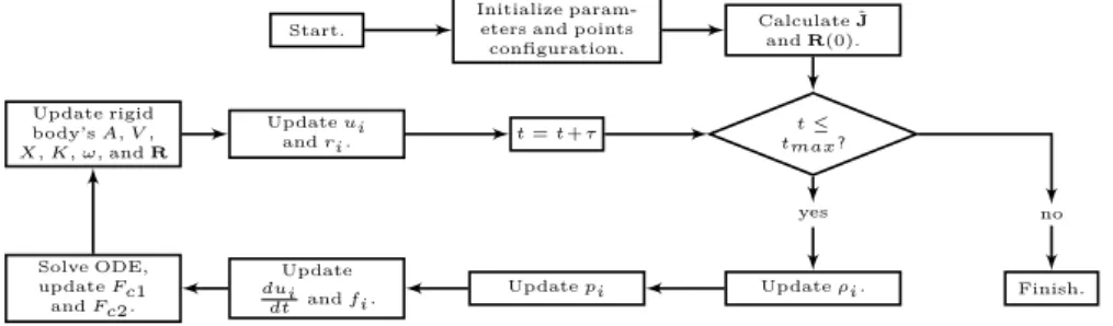
The algorithm of the simulation can be seen on Figure 3.

(9)

Start.

Initialize parameters and points configuration.

CalculateJˆ andR(0).

Update rigid body’sA,V, X,K,ω, andR

Updateui

andri. t=t+τ t≤

tmax?

yes no

Solve ODE, updateFc1 andFc2.

Update dui

dt andfi. Updatepi Updateρi. Finish.

Figure 3: The algorithm of the simulation.

4 Results and Discussions

4.1 Simulation Set-up

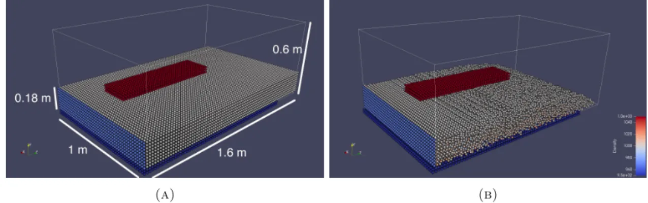
We choose the inclination angle of the ocean wave relative to the world horizon to be ϕ = 10^◦ with the ocean wave moves with a constant velocity V_f = 2.5. The frame of the system’s domain is located at the upslope part of the ocean wave and moves together with the ocean wave (see Figure 1a). Gravity acts as an external body force per unit mass is set to beg=−9.81(0,cosϕ,sinϕ). The size of the domain is set to be 1×0.6×1.6 with the depth of the water is0.18. The system has a periodic boundary condition in x-axis, non-zero Dirichlet boundary on some parts of left boundary by using ghost points (rendered with light blue color in Figure 4a) for−0.3≤y <−0.12, bottom boundary is also set to be a non-zero Dirichlet boundary by using a non-moving boundary points (rendered with dark blue color in Figure 4a) for−0.8 ≤z <0.56, and free boundary in right boundary, top boundary, left boundary for−0.12≤y <0.3, and bottom boundary for 0.56≤z≤0.8. Take a note that the origin point is located at the center of the domain. The size of the rigid body is0.2×0.06×0.8. The rigid body is represented by red points in Figure 4a. Initially, the center of mass of rigid body is positioned at(0,−0.04,−0.27).

The density referenceρ0 is set to beρ0 = 1000, while the density of the rigid body isρb = 100. The fluid is initialized to have an initial velocityui(0) =Vf = 2.5 toward+z-axis, and initial density to beρi(0) =ρ0 for all fluid points r_i. By our choice of piecewise cubic kernel (7) as a mollifier function and choose the points to be initialized in a regular grid with a distancehin each axis, Vi andmi for all points are Vi = 8×10⁻⁶ and mi = 0.008. We set the parameter of the kernel function to be h = 0.02. Time step size is set to be τ= 0.0005with the speed of sound is chosen to bec= 20. The positions of contact point 1 and contact point 2 arerc1= (0., −0.03, −0.4)andrc2= (0., −0.03, 0.4), respectively, relative to the position of the center of mass of the rigid body.

Free boundary condition is implemented by changing the type of any fluid points leaving the domain into a ghost point which its velocity does not change with time and its density always equal to the reference density ρ0, but still interacts with other points. If a ghost point enters the domain, it will be marked as a normal fluid point again. But if it leaves the domain farther thanh, the point will be removed from the simulation.

Before we run the actual simulation, we run the “relaxation” process to stabilize the flow of the water up to t= 1.5. The initial condition after relaxation can be seen on Figure 4b.

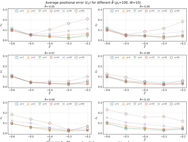
To find the best combination of parameters, we run simulations with each combination ofθ˜∈ {−0.05,−0.06,

−0.07,−0.08,−0.09,−0.1}andµ∈ {1,2,5,10,20,50} for eachZ˜∈ {−0.6,−0.5, −0.4,−0.3,−0.2}. We take

(10)

(a) (b)

Figure 4: (A) The initial configuration of the system, (B) The configuration of the system after the relaxation process.

the average of positional error for a given combination of parameters(µ,θ,˜ Z)˜ for the whole simulation time,

ϵZ(µ,θ,˜ Z) :=˜

∑Υ m=0

Z(µ,θ,˜ Z, mτ˜ )−Z˜

Υ + 1 ,

whereΥis a number of time steps. The graph of the average positional error can be seen in Figure 5. Then we take the average of error over all parametersZ,˜

ϵZ(µ,θ) :=˜

∑

Z˜∈Z˜setϵZ(µ,θ,˜ Z)˜

#Z˜set

, Z˜set={−0.6,−0.5,−0.4,−0.3,−0.2},

and calculate the cumulative error for eachθ˜andµ. The average of error over all parameters Z˜ can be seen in Table1.

Table 1: Table of the average of error over all parametersZ˜and its cumulative errors for eachθ˜andµ.

µ\θ˜ −0.05 −0.06 −0.07 −0.08 −0.09 −0.10 C.E.

1 5.74e-02 5.81e-02 5.33e-02 5.80e-02 5.98e-02 5.44e-02 3.41e-01 2 5.30e-02 5.13e-02 5.08e-02 4.67e-02 5.48e-02 5.94e-02 3.16e-01 5 5.02e-02 5.29e-02 4.62e-02 4.76e-02 4.53e-02 4.89e-02 2.91e-01 10 5.97e-02 5.13e-02 4.66e-02 4.65e-02 5.08e-02 6.29e-02 3.18e-01 20 8.47e-02 7.04e-02 5.07e-02 5.07e-02 6.92e-02 9.33e-02 4.19e-01 50 1.28e-01 1.08e-01 7.15e-02 7.00e-02 9.97e-02 1.72e-01 6.49e-01 C.E. 4.33e-01 3.92e-01 3.19e-01 3.20e-01 3.80e-01 4.91e-01

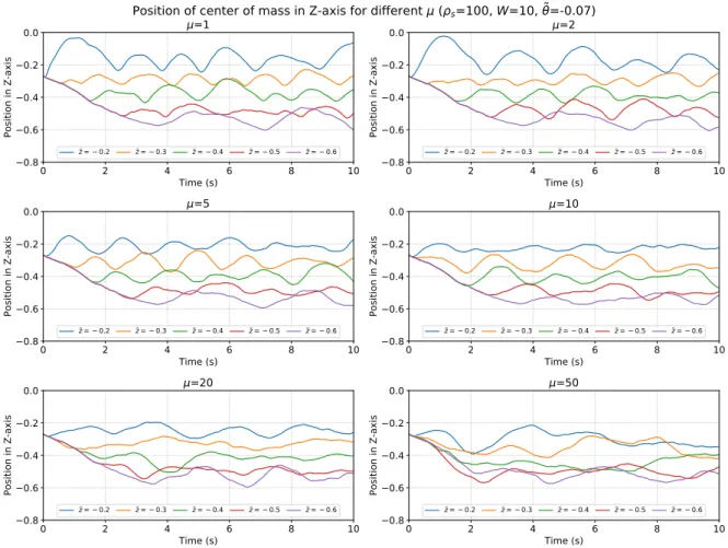
As we can see from Table 1, θ˜ = −0.07 and µ = 5 give the smallest cumulative errors for each θ˜ and µ, respectively. Now let us see more in detail the simulation results forθ˜=−0.07in Figure 6.

As we can see from Figure 6, there are some oscillations of the position of the rigid body. As the value ofµ is increasing, the amount of oscillations is dampened. The oscillation is occurred because of the wrong choice of theµ compared to the actual value µ of the system. As the value ofµ is increasing (we assume that it is getting closer to the actual value of µas it increases), the oscillation is dampened. Besides, our previous assumption thatµ_v =µ_z= 0is also not correct in the real case. As we choose the frame to be inclined relative to the world horizon, the gravity influences the velocity of the flow, yielding different velocities at different positions, and leading to the dependency of the drag to the position. Since now the flow is not constant, the drag also depends on the velocity of the flow, leading to the dependency of the drag to the velocity as well.

We also notice that we face another problem: shifted stable position. This problem is due to the wrong choice ofθ. We set˜ θ˜to be the same value for the whole simulation. Adding an additional ODE control for θ˜will

(11)

0.6 0.5 0.4 0.3 0.2 Z

0.0 0.1 0.2 0.3

Z

=-0.05

=1 =2 =5 =10 =20 =50

0.6 0.5 0.4 0.3 0.2

Z 0.0

0.1 0.2 0.3

Z

=-0.06

=1 =2 =5 =10 =20 =50

0.6 0.5 0.4 0.3 0.2

Z 0.0

0.1 0.2 0.3

Z

=-0.07

=1 =2 =5 =10 =20 =50

0.6 0.5 0.4 0.3 0.2

Z 0.0

0.1 0.2 0.3

Z

=-0.08

=1 =2 =5 =10 =20 =50

0.6 0.5 0.4 0.3 0.2

Z 0.0

0.1 0.2 0.3

Z

=-0.09

=1 =2 =5 =10 =20 =50

0.6 0.5 0.4 0.3 0.2

Z 0.0

0.1 0.2 0.3

Z

=-0.10

=1 =2 =5 =10 =20 =50

Average positional error ( Z) for different ( s=100, W=10)

Figure 5: The graphs of the average positional error.

help the board to move slowly to the desired position after the “pre-stable condition” is achieved. In a real case, θ˜is learned by the surfer as the “target inclination angle” if they want to move the surfing board to a desired point along the ocean wave. Finding correct parameters for an additional ODE control forθ˜can be seen as an effort to learn those target inclination angle if the position of the surfing board is off from the desired position.

If we looks closer and compare Figure 1b with Figure 6, we can see that the oscillations on the direct solver is on the inclination angle and velocity, while in the SPH simulation the oscillations occur on the position.

This problem happens because of the delayed response in the SPH simulation. The change of the inclination angle from the ODE control cannot be translated instantly into the change of the inclination angle in the SPH simulation.

5 Summary

An ODE control is successfully implemented into a coupled inviscid fluid-rigid body SPH simulation in an attempt to control the movement of the surfing board. For our system, the best values for θ˜ and µ are θ˜=−0.07and µ= 5. Althoughµ= 5does give the best result, it does not mean the actualµof our system is equal to 5. Several problems still occur, such as oscillations and shifted stable position. The oscillation problem can be solved by finding correct values for all µ, µv, and µz. Adding an additional control for θ˜ will solve the shifted stable position problem by nudging the surfing board slowly toward the desired position after the system is almost stable. The delayed response from the SPH simulation also has a responsibility on the oscillations problem, since the change of the inclination angle from the ODE control cannot be translated instantly into the SPH simulation.

(12)

0 2 4 6 8 10 Time (s)

0.8 0.6 0.4 0.2 0.0

Position in Z-axis

=1

Bibliography

[1] John F. Wendt.Computational Fluid Dynamics. Springer-Verlag, Berlin Heidelberg New York, 2nd edition, 1995.
[2] G.B. Folland.Real Analysis: Modern Techniques and Their Applications. Pure and Applied Mathematics:
A Wiley Series of Texts, Monographs and Tracts. Wiley, 2013. ISBN 9781118626399. URL https:
//books.google.co.jp/books?id=wI4fAwAAQBAJ.
[3] J. J. Monaghan and J. C. Lattanzio. A refined particle method for astrophysical problems. Astron.
Astrophys., 149:135–143, 1985.
[4] G. K. Batchelor. An Introduction to Fluid Dynamics. Cambridge University Press, 2000.
[5] J. J. Monaghan. Smoothed particle hydrodynamics. Rep. Prog. Phys, 68:1703–1759, 2005.
[6] Igor P. Omelyan. Algorithm for numerical integration of the rigid-body equations of motion. Physical Review E, 58(1):1169–1172, July 1998.