(
Memoirs of the Faculty of Education and Human StudieS) Akita University (Natural Science)
63, 15 - 19 (2008)
Roots of One Parameter Modular Equations of j (z)
Hideji Ito*
\Ve make experimental observation about one parameter modular equations <I>p(X, XP) = 0 of the elliptic modular function j(z), especially about their factorizations and behavior oftheir roots.
(i) deg if>p(X, XP) = p2 + P - 1, d p 2+ p _l = 744 x p
1 Introduction
The classical elliptic modular function j (z) satisfies the so-called modular equation
if>n(j(z),j(nz)) = 0,
Explicitly, set if>p(X, Y)
I: aik Xiyk , and if>p(X, XP) readly have
Xp+l + yp+l +
= I: dkX k. Then we
for each natural number n, where the if>n(X, Y) are certain polynomials with gigantic coefficients (for large n) in Z[X, Y]. An estimate of the magnitude of coefficients is given by P.Cohen [2]. Hereafter we consider the case n = p (odd prime) exclusively unless othewise explicitly stated.
There is a long history of explicit calculation of modular polynomials if>p(X, Y). I myself computed them for all p < 200 around 2000. It seems the most extensive calculation was done by M.Rubinstein (with the aid from G.Seroussi) as far as p < 360. The result is on the web [11], although the method of calcula- tion is apparently not published yet. More recently an entirely different method is given by Charles and Lauter [1]. They don't use q-expansions of .j(z) but rely on the grapf of supersigular elliptic curves over finite fields. (They even made their algorithm a US patent. [4])
::"ow putting Y = XP in if>p(X, Y), we get polyno- mials in one variable if>p(X, XP). In this paper, we will call them one parameter modular polynomials and the equation if>p(X, XP) = 0 will be called one parameter modular equation. This is the object of study in this paper.
* The author was partially supported by Grant-in-Aid for Scientific Research (C)(2), No.1264007, Japan Society for the Promotion of Science.
(ii) if k = n+mp(m = 0 or 0 < n,m < p, (n,m) i-
(1,1)), then we have d k = a nm ; also we have d p + 1 =
all + 1, dkp = ap,k-l + aO,k (1 :::; k :::; p).
They are used by Kaneko [10] to give a reduction of my observation [5] to yet another numerical facts.
But he considered them solely in characteristic p. In contrast we consider them primarily over C, the usual complex number field.
Our present study begins with the investigation of the magnitude of coefficients a nm . Actually the biggest coefficient is usally aOO when it is not O. When aOO is 0, the biggest one is a20 or al,l' See the table in the appendix 1. \Vith our aim in mind, we are led to examine the solutions of if>p(X, XP) = 0, because the coefficients of a polynomial f(X) in one variable are closely related with the solutions of the equation f(X) = 0 and the d k and the a nm are much the same as noted in (ii) above. By numerical and graphical calculation on computer we found that very striking patterns would emerge. As yet, we are unable to give proof of our observations. But I think it worthwhlie to record them here to allow everyone interested to examine our findings and pursue the investigation.
Most parts of the present paper were first reported
in [8] which was written in Japanese. It contains the
graphics of the distribution of roots of if>p(X, XP) = 0
for p :::; 61 and numerous tables of computed values
relevant to our theme.
2 Facterization of <pp(X, XP)
Let <I>~3)(X, Y) be the modular polynomial of j(Z)1/3
which is a modular function with respect to r(3) (see Ito [6]). Using it, we have a factorization of <I>p(X, XP) as follows.
Theorem 2.1
(i) If p == 1 (mod 6), then we have
Here F p, G p E Z[X] are determined by
<I>~3) (X, XP) = pX 2Fp(X 3),
<I>~3) (X, (XP)<I>~3) (X, (2 XP) = X 4 Gp(X 3), where ( is a third root of unity(i- 1) and we have
deg Fp(X) = (1/3)(p2 + P - 5), degGp(X) = (2/3)(p2 + P - 2).
(ii) If p *- 1 (mod 6), then we have
Here F p , G p E Z[X] are determined by
<I>~3) (X, XP) = pFp(X 3),
<I>~3) (X, (XP)<I>~3) (X, (2 XP) = Gp(X 3),
and we have
degFp(X) = (1/3)(p2 + P - 3), degGp(X) = (2/3)(p2 + p).
Proof. We first recall the relation
p ==
and h,o = o. So we obtain
<I>~3) (X, XP) = X 2(Xp-1 + 2..: fabxa+pb-2) Since p - 1 == a + pb - 2 == 0 (mod 3), we can write <I>~3) (X, XP) = X 2S(X 3) for some polynomial S(X) E Z[X]. Also congruence relation <I>p(X, Y) ==
(XP - Y)(X - YP) (mod p) gives us <I>~3) (X, XP) == 0 (mod p). Hence we get the final form <I>~3) (X, XP) =
pX 2Fp(X 3) for some polynomial Fp(X) E Z[X].
Also from this we easily see that we can write
<I>~3) (X, (XP)<I>~3) (X, (2 XP) = X 4 Gp(X 3) for some
Gp(X) E Z[X], As for degrees of Fp(X) and Gp(X) , note that <I>~3) (X, XP) = p2 + P - 3.
The case p *- 1 (mod 6), that is, p == 2 (mod 3) can be dealt with similarly.
Computer calculation indicates that the polyno- mails Fp(X) , Gp(X), Fp(X) and Gp(X) are always irreducible over Z.
3 Distribution of the roots
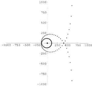
Figure 1 shows the distribution of most roots of
<I> 37 (X, X 37 ) = O.
1000
7S0
SOO
<I> P ' (X 3 y 3) = <I> (3)
p '(X Y)<I>(3)
p " < , .(Y (Y)<I>(3) P (Y
-L,~i 2y) (See Elkies [3] or Ito [6].) Since the polynomial
<I>~3) (X, (Y)<I>~3) (X, (2y) is invariant under the galois action of Q(() = Qh/=3) it is contained in Z[X, :Y].
Put <I>~3)(X,Y) = Xp+1 + yp+1 + L.~,b=ofabxayb.
We know fab = ° unless a+pb == p+ 1 (mod 3). (See ibd.) So if we put Y = XP, we have
2S0
-10'-=0-=-0-_-='7::C S 0:----=-50;C;:' ' " 0 §""::° ~\ oc
0
..
l.
• •-25~·~····
•-750
-1000
750 1000
P
<I>~3) (X, XP) = Xp+1 + Xp(p+1) + 2..: fab xa+pb
a,b=O
Here in the sum the pair (a, b) runs through the range ° ~ a, b ~ p with the condition a + pb == p + 1 (mod 3), (a, b) i- (0,0). (Kote that
fpp = -1.)
Figure 1: Distribution of roots of <P37(X, X37) = 0 (almost all)
The figure strongly suggests the existence of what we might call the "root curve" of <I> 37 (X, X 37 ) = O.
The roots not appearing in the figure are 6 in number
and it seems they sit on the extension of the branch
of the root curve.
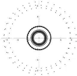
Near the origin a lot of roots accumulate. Figure 2 shows their behavior.
°6
00
0 ' ,
.. -6 -4
0, ,
'0
Figure 2: Distribution of roots of <P37(X,X37 ) = 0 (-7 < Re(X)< 7)
To see more clearly we give the grapf in the range IRe(X) I < 2.5 in Figure 3.
2, ,
0'
Figure 3: Distribution of roots of <P37(X, X 37 ) = 0 (-2.5 < Re(X) < 2.5)
In this paper we loosely use the term the root curve C p of pp(X, XP) = 0 to mean the hypothetical curve or the distribution of its roots itself. From experi- mental calculation such as the above we made several observations. They are summarized as follows,
(1) Except near the origin, there is quite a similarity among Cp's for different p. Indeed we suspect the existence of lim C p as a specific curve.
(2) ~ear the origin, there are a number of "rings"
(a kind of "spectrum"). The number becomes large as p becomes large. In the range -2.5 < Re(X) < 2.5, the number is 1 for p ~ 11, 2 for 13 ~ p ~ 17, 3 for 19 ~ p ~ 29, 4 for p = 31, 5 for p = 37. For more bigger p, we are not sure about their number, because we cannot decide whether it is a single ring or two (or many more ) rings that are too close to distiguish.
(Compare Fig.2 and Fig.3.)
(3) The absolute values of the roots are always greater than 1 ( except for the trivial one X= 0 in case p == 1 (mod 6)). On the other hand, the maxi- mal absolute value of the roots increase slowly. They are comparatively small. For example, for p = 61 the maximal value is approximately 7223.
(4) The most remarkable phenomenon we found is this: except in the trivial case, there is only one real root of pp(X, XP) = 0, and if p be- comes large those values approach quite fast to -5.5459008793608518348144419091322705411400···
monotonously from below. (This fact somewhat supports our conjecture made in (1) even near the origin in some modified way.)
(5) What is the value z for which j(z) is the above mentioned unique root? Evidently z is on the line Re(z) = -,} closeto(= (-1+0)/2. We found an approximate value of z = ~1/2+0.916953958i, where
i=A.
(6) If j (z) satisfies Pp(j(z), j (z )P) = 0, then j (z)P must be of the form j (a z) for some a in the set
{( ~ ~), (~ ~) (0 ~ k ~ p - I)}.
Numerically we found for the value z in (5), a = (~ ; ) for c = (p + 1) /2.
(7) The theorem 2.1 says that the polynomial pp(X, XP) has two factors (except for the trivial one).
But the root curve C
pdoes not split into two parts in any obvious way. Indeed both factors have similar root curves, naturaly with fewer points than Cpo See Figure 4 for the first factor of P37(X, X 37 ). Also we note that the unique real root mentined in (4) always belongs to the first factor.
Remark 3.1 \Ve obtain other root curves corre- sponding to some modular functions such as t 2A or
t2B, the notation being the same as in [9]. See ap-
pendix 2 for their graphics.
250 '
..
~. .
-1000-~-~--500 ----=-25~-~-~0---:-sOO
750-1"000-1000
Figure 4: Distribution of roots of the first faetor of
<I>37(X,X37 ) = a (almsost all)
Figure 5: Distribution of roots of the first factor of
<I>37(X, X37) = a (-7 < Re(X)< 7)
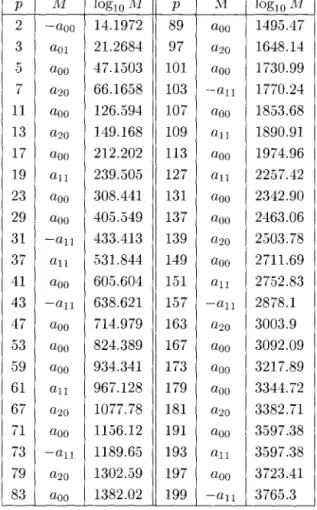
Appendix 1. Maximal values of the absolute values of the coefficients of <pp(X, Y)
In the range p :s 199, if p == 5 mod 6 then laool is maximal, while if p == 1 mod 6 then as is well known
aoo = 0 ( in fact, in this case we have aoo = ala = 0 (see Ito [7]) and la201 or lalll is maximal. We denote by M the maximal value of the laij I in the following table.
p M lOglO 1'v1 P M lOglO Al
2 -aOO 14.1972 89 aOO 1495.47 3 aOl 21.2684 97 a20 1648.14 5 aOO 47.1503 101 aOO 1730.99 7 a20 66.1658 103 -all 1770.24 11 aOO 126.594 107 aOO 1853.68 13 a20 149.168 109 all 1890.91 17 aOO 212.202 113 aOO 1974.96 19 all 239.505 127 all 2257.42 23 aOO 308.441 131 aOO 2342.90 29 aOO 405.549 137 aOO 2463.06 31 -all 433.413 139 a20 2503.78 37 all 531.844 149 aOO 2711.69 41 aOO 605.604 151 all 2752.83 43 -all 638.621 157 -all 2878.1 47 aOO 714.979 163 a20 3003.9 53 aOO 824.389 167 aOO 3092.09 59 aOO 934.341 173 aOO 3217.89 61 all 967.128 179 aOO 3344.72 67 a20 1077.78 181 a20 3382.71 71 aOO 1156.12 191 aOO 3597.38 73 -all 1189.65 193 all 3597.38 79 a20 1302.59 197 aOO 3723.41 83 aOO 1382.02 199 -all 3765.3
(\Vhen a •• is negative we write
- 0 . .in the above table.)
Appendix 2.
Modular polynomials of order p of t 2A ( t 2 B, respec- tively) are denoted by <p~t2A) (<p~t2B), respectively).
150"
100
•S~-' • • •
.
'----~,-
>---~--'-'
- - - ' - - - ' - - - --100 :--.50
---@)-
50 •• '100 150 200~ ~(J -• • • •
-150'e
Figure 6: Distribution of roots of<I>~t12A)(x,X31) = a
(all)
-18-
15 20-
:
.
~ .::::.i:: ...:::
-20
-is -10 -
-5 ;...: '.
·5 10 - 15··f···· .
-5c
-10
20
[10] JVLKaneko, Ito's observation on coefficients of the modular polynomial, Proc. Japan Acad. 72, Series (A) (1996),95-96.
[11] M.Rubinstein, http://www.math.uwaterloo.ca/
-mrubinst/modularpolynomials/phiJ.html
-20