in the Yellow Sea

(1)

九州大学学術情報リポジトリ

Kyushu University Institutional Repository

黄海におけるラグランジュ粒子運動の数値シミュレーション

王, 彬

https://doi.org/10.15017/1398417

出版情報：Kyushu University, 2013, 博士（理学）, 課程博士バージョン：

権利関係：Fulltext available.

(2)

Numerical Simulation of Lagrangian Particles Motion

in the Yellow Sea

Bin Wang

July 2013

(3)

Numerical Simulation of Lagrangian Particles Motion

in the Yellow Sea

A Dissertation for the Doctoral Degree of Science in Kyushu University

By

Bin Wang

Earth System Science and Technology,

Interdisciplinary Graduate School of Engineering Sciences, Kyushu University

July 2013

(4)

Abstract

The Lagrangian particles motions in the Yellow Sea are studied on the basis of a series of high-resolution numerical experiments. That is because, comparing with the Eulerian framework, the Lagrangian phenomena of the circulation have not been well examined in this area. For instance, the mechanisms and the predictions of the green-tide events, which have occurred frequently in the southwestern Yellow Sea during recent summers, have been trended unsatisfactorily.

In the first half of this study, the responses to tidal and/or wind forces of Lagrangian trajectories and Eulerian residual velocity field in the upper layers of the southwestern Yellow Sea are investigated. All of the characters of the water masses, including the thermocline and the position of the surface and subsurface water masses, are simulated well by the numerical model, implying that the present model has captured the essential dynamics of the current systems. The simulated tidal harmonic constants agree well with observations and existing studies. The numerical experiment reproduces the long-range southeastward Eulerian residual current over the sloping bottom around the Yangtze Bank which also shown in previous studies.

However, the modeled drifters deployed at the northeastern flank of Yangtze Bank in the simulation move northeastward, crossing over this strong southeastward Eulerian residual current rather than following it. Additional sensitivity experiments reveal that the influence of the Eulerian tide-induced residual currents on Lagrangian trajectories is relatively weaker than that of the wind driven currents in the upper layer of the southwestern Yellow Sea. This result is consistent with the northeastward movement of ARGOS surface drifters actually released in the same region.

Further experiments suggest that the quadratic nature of the bottom friction is the crucial factor, in the southwestern Yellow Sea, for the weaker influence of the Eulerian tide-induced residual currents on the Lagrangian trajectories. The simulation result demonstrates that the Lagrangian trajectories do not follow the Eulerian residual velocity fields in the shallow coastal regions of the southwestern Yellow Sea.

In other words, the Lagrangian residual current in representing the inter-tidal mass transport is more accurate comparing with the Eulerian residual velocities.

(5)

In the second part of this thesis, combined with the in situ hydrographic observation data from the Korea Oceanographic Data Center (KODC), significant southward seasonal migrations of Yellow Sea Bottom Cold Water (YSBCW) are simulated successfully. The possible source and the 3-D pathway of the YSBCW are quantitatively calculated using the two-way Lagrangian particle tracking method (PTM). The dynamical factors of the YSBCW seasonal migration are also investigated by numerical modeling.

The trajectories of the modeled drifters show that, the subsurface cold heavy water masses, from the northern part of the Yellow Sea and the southern part of the Sea of Bohai, sink into deeper layers gradually with the southward movement since spring to summer. The southward extensions gradually gather speed from February to July or August. Until September or early of October, the cold-water masses reach the southernmost location; they even can affect the southwest region of Cheju Island.

Furthermore, the results of the additional sensitivity experiments demonstrate that the tide-induced residual currents under baroclinic conditions are the primary forcings for the deep circulation in the Yellow Sea. The summer southerly wind and strong solar radiation, causing the inter-annual variations of the currents, are also demonstrated to effectively contribute to the southward migration of the YSBCW.

While, the effect from the Changjiang (Yangtze) River discharge is insensitive. On the other hand, the seasonal migrations of the YSBCW are minor affected by the meteorological forcings during previous wintertime.

Consequently, the simulation results suggest that the Lagrangian trajectories do not follow the Eulerian residual velocity fields in the shallow coastal regions. In other words, streamlines of the Eulerian residual velocities and the Lagrangian trajectories (path lines) can be significantly different in coastal seas, and the difference should not be ignored as demonstrated in this study. The Lagrangian residual circulation should be considered as the base of the dynamics in a coastal sea. To accurately embody the mass transport in the shallow region of the Yellow Sea, the Lagrangian framework of circulation should be paid more attention, comparing with the Eulerian residual velocity.

(6)

List of Figures

Figure 1.1. Topography in the Bohai Sea, the Yellow Sea and the East China Sea... 19 Figure 1.2. Observed T-S diagrams of KODC data set over 20 years from 1991 to

2010: (a) in February, (b) in August... 20 Figure 1.3. Schematic representations of the circulation systems of the China Seas

from Guan (1994) during winter (a) and summer (b) times, respectively... 21 Figure 2.1. Model domain and topography; the thick solid line shows the initial

location of artificial drifters (the contour interval is 10 m). Black dots are the locations of the tidal observation stations... 43 Figure 2.2. Trajectories of surface ARGOS drifters from Li (2010) in the summer of

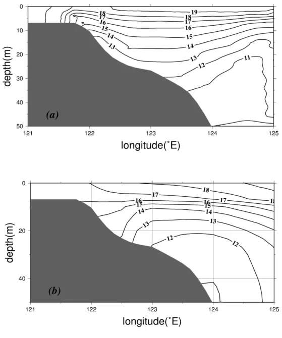
2009 (Fig.3.2 in that paper) ... 44 Figure 2.3. Simulated (a) and observed (b) climatological vertical temperature

distributions along the 33°N sections in June... 45 Figure 2.4. Simulated (a) and observed (b) climatological vertical temperature

distributions along the 35°N sections in June... 46 Figure 2.5. Co-tidal charts simulated with homogeneous water. Solid and dashed

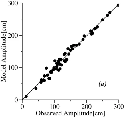
lines show the distributions of amplitude (in meters) and phase lag (in degrees and referred to 120°E), respectively... 47 Figure 2.6. Comparison between the observed and simulated M2 tide harmonic

constants (a) amplitude and (b) phase. Stations are shown as black dots in Figure 2.1... 48

(9)

Figure 2.7. (a) Simulated Eulerian tide-induced residual currents in TQ and (b) simulated circulation in WTQ at a depth of 15 m during June... 49 Figure 2.8. Streamlines superimposed on the magnitudes of velocities (m/s)

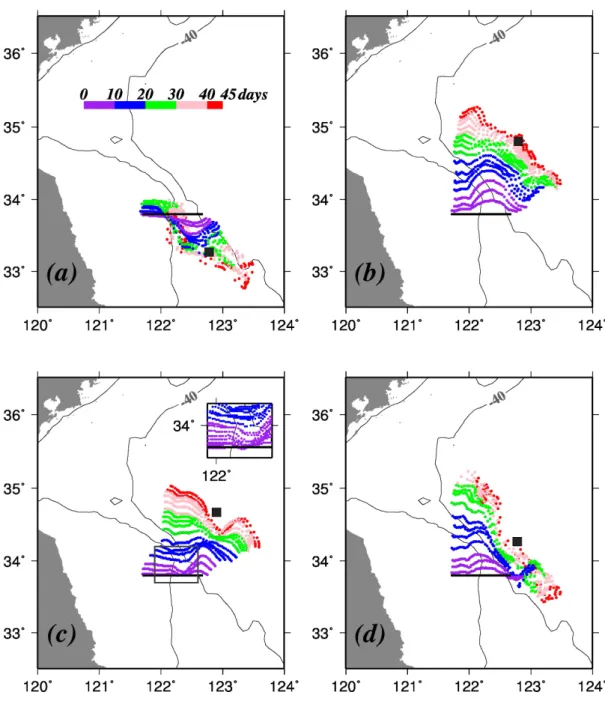
calculated based on the Eulerian residual fields in Figure 2.7. The magnitude of velocity smaller than 0.01 m/s is not shown... 50 Figure 2.9. Trajectories of the artificial drifters plotted with 2.5-day interval (a) in

TQ, (b) in WQ, (c) in WTQ, with 1-day interval in the small box area, (d) the linear combination of WQ and TQ. The square indicates the final weighted center of the drifters 45 days after release... 51 Figure 2.10. Trajectories of the artificial drifters plotted with 2.5-day interval (a) in

WTL and (b) the linear combination of WL and TL... 52 Figure 2.11. Trajectories of the artificial drifters plotted with 2.5-day interval in the

experiment forced by the tidal forcing and the wind stresses from May to June in 2009... 53 Figure 2.12. Monthly wind stress vectors during June obtained from JRA-25

reanalysis data. (a) climatological mean ones, (b) in 2010... 54 Figure 2.13. Trajectories of the artificial drifters plotted with 2.5-day interval (a) in

RTQ, (b) the linear combination of RQ and TQ, (c) in RTL, (d) the linear combination of RL and TL... 55 Figure 3.1. Model domain and topography. The dots present the observation stations

of KODC data set. The in situ observations from stations A and B are used to identify the time series of simulated temperature... 84

(10)

Figure 3.2. Schematic diagrams of two-way PTMs referred from Isobe et al. (2009).

S and R present source and receptor, respectively. (a) FIT calculation of the particles, (b) BIT calculation of the particles from receptor, (c) elimination between the source candidates... 85 Figure 3.3. Schematic diagram of the horizontal projection of weight ellipsoid.

Points A and A’ denote the initial location and the returned location after two-way PTMs calculations, respectively. xi and yi present the deviation distances in zonal and meridional direction, respectively. θ1, σ1 and σ2 are calculated from formulas 3.1 to 3.3, respectively... 86 Figure 3.4. Temperature distributions at 50 m depth from KODC data in 2008: (a)

February, (b) April, (c) June and (d) August. The contour interval is 1°C... 87 Figure 3.5. Same as Figure 3.4, but for 2009... 88 Figure 3.6. Same as Figure 3.4, but for 2010... 89 Figure 3.7. Horizontal temperature in February of 2009: panels (a1) and (b1)

present the simulated results at sea surface and 50 m, respectively; panels (a2) and (b2) present the remote sensing and in situ observations at sea surface and 50 m, respectively. The contour interval is 1°C... 90 Figure 3.8. Same with Figure 3.7, but for April... 91 Figure 3.9. Same with Figure 3.7, but for June... ⁹² 58 Figure 3.10. Same with Figure 3.7, but for August... 93

(11)

Figure 3.11. Vertical distribution of temperature along 35°N section in June: (a) the simulated result in 2009, (b) the observation data of 2009 from KODC and (c) the GDEM climatological temperature. The contour interval is 1°C... 94 Figure 3.12. Time series of the simulated temperature at 50 m of the stations

presented in Figure 3.1 in 2009. Star marks present the KODC in situ observation data... 95 Figure 3.13. Temperature differences between August and February of 2009 at 50 m

depth: panel (a) and panel (b) present the simulated result and the observation, respectively. The contour interval is 1°C... 96 Figure 3.14. Figure 3.14. Locations of (upper panels) all of the modeled drifters and

(lower panels) those drifters could return inside the weight ellipsoid: (a) at end of February (initial locations), (b) at end of July by the BIT calculation and (c) at end of February by the FIT calculation. The size of dot in panel (a) presents the layers of the drifters... 97 Figure 3.15. Horizontal distributions of the modeled drifters at end of February and

October in 2009. The asterisks and squares present the horizontal and vertical locations of the weighted centers of modeled drifters in 2008 and 2009, respectively... 98 Figure 3.16. Monthly meridional displacements of the modeled drifters in 2009.

Positive value (blue dots) means northward and negative value (red dots) means southward... 99 Figure 3.17. Total southward distances during June and July in each experiment... 100

(12)

Figure 3.18. Comparisons of the southward displacements during May and June in the year of 2008 and 2009...

101

Figure 3.19. Wind stress of JMA dataset in May: panel (a) and panel (a) present that in 2008 and 2009, respectively... 102 Figure 3.20. Same with Figure 3.19, but for June... 103 Figure 3.21. Short wave radiation of JMA dataset in May: panel (a) and panel (a)

present that in 2008 and 2009, respectively. The contour interval is 10W/m²...

104

Figure 3.22. Same with Figure 3.21, but for June... 105

(13)

List of Tables

Table 2.1. Final mean meridional displacement of the artificial drifters and the

area-averaged magnitude of the bottom momentum flux in each experiment.. 56 Table 2.2. Final mean meridional displacement of the artificial drifters in the

realistic cases... 57 Table 3.1 Values of the variables and constants for calculation of surface net heat

flux in formula (3.3), which is referred from Hirose et al. (1999). (TABLE 1. in that paper)...

106

Table 3.2 List of each experiments and forcing... 107

(14)

List of Abbreviations

SST: sea surface temperature

SSS: sea surface salinity

SAT: surface air temperature

YSBCW: the Yellow Sea Bottom Cold Water

PYSBCW: the precursor of the Yellow Sea Bottom Cold Water

YSWC: Yellow Sea Warm Current

CDW: Changjiang Diluted Water

TWC: Tsushima Warm Current

ADCPs: Acoustic Doppler Current Profilers

KODC: Korea Oceanographic Data Center

NFRDI: National Fisheries Research and Development Institute

POM: Princeton Ocean Model

JRA-25: the Japanese 25-year re-analysis (JRA-25) dataset

GDEM: Generalized Digital Environmental Model

(15)

MOODS: Master Oceanographic Observation Data Set

BMF: the bottom momentum flux

GSM: Global Spectral Model (GSM) dataset

JMA: Japan Meteorological Agency

MGDSST: Merged satellite and in situ data Global Daily Sea Surface Temperatures

PTM: particle tracking method

BIT: backward-in-time

FIT: forward-in-time

(16)

Chapter 1 Introduction

(17)

The Yellow Sea is a semi-enclosed marginal sea of the western North Pacific located between the Chinese mainland and Korean Peninsula connecting with Bay of Bohai from the north and East China Sea from the south.

The bottom topography of Yellow Sea is highly variable, containing the well-developed continental shelf along the coast region and the north-south elongated Yellow Sea central trough with its axis closer to the Korean coasts than to the Chinese coasts. The near-shore water depths of the western part of Yellow Sea are generally shallow, including the broad Yangtze Bank which shallower than 20 m within around 50km off the east coasts of China. While, the north-south Yellow Sea trough, with the maximum depth exceeding 90 m, is flanked from the border between Yellow Sea and Bohai Sea to the continental shelf break at southeast of Cheju Island, which is considered as an important conduit of the water exchange between Yellow Sea and the East China Sea (Figure 1.1). The complicated controlling effects of the variable bottom topography were suggested to confine the circulation in the southwestern Yellow Sea (Wang et al., 2013).

The hydrological characteristics of the circulation and the thermal structures in the Yellow Sea have strong seasonal variation associated with the Asian monsoon.

During wintertime, the tough cold northwesterly wind occupies over the entire Yellow Sea due to the Siberian high-pressure system. In the meantime, the sea surface temperature (SST) in wintertime is roughly 2 °C to 6 °C warmer than the surface air temperature (SAT). The Yellow Sea loses the heat to the atmosphere from the sea surface. The upward net heat flux between the air-sea interfaces,

(18)

combining with the strong northerly wind, generates the strong vertical turbulence mixing. The winter circulation of the Yellow Sea performs a perfect barotropic property. The temperature of Yellow Sea is basically vertical homogeneous at this time. The low temperature and the low salinity Yellow Sea Water that is the precursor of the Yellow Sea Bottom Cold Water (PYSBCW), and the relatively high temperature and high salinity water mass from the Kuroshio origin intruding into the interior of the Yellow Sea roughly along the deep central through, which is the so-called Yellow Sea Warm Current (YSWC), are the significant hydrological characteristics in the Yellow Sea during wintertime. Figure 1.2a illustrates the observed T-S diagrams in February over 20 years from 1991 to 2010, which is obtained from the Korea Oceanographic Data Center (KODC). It clearly reveals these two different water types. The two different water masses form a strong surface-to-bottom thermohaline front running from west to east in the region west of Cheju Island (Lie, 1986).

From the end of winter, the wind directions are highly variable, due to the weakening of the Siberian high-pressure system. From late of May or early of June, the summer surface atmospheric low-pressure system begins to form over Asian region, which initially locate at the north of the Yellow Sea, and produces weak westerly winds (Chu et al., 1997). The circulation in the Yellow Sea is relatively quiescent during May, followed by the defined summer mode. In late of June, the low-pressure center starts to migrate westward. The southwesterly monsoon occurs, which is dominated during the whole summer season. Despite the summer

(19)

low-pressure system is in progress, the averaged surface wind speed over the central Yellow Sea in summer is less than 4 m/s, which is obviously weaker than that during wintertime (Watts, 1969; Van Loon, 1984).

In summer, the waters of the Yellow Sea have a wider range of temperature and salinity comparing with those in wintertime, reflecting the effects of the surface heating, the heavy precipitation and the abundant fresh water discharge. The strong and clearly visible stratifications during warm season in the Yellow Sea indicate that the baroclinic circulation is prevailing.

Figure 1.2b is the observed T-S diagrams of KODC data set in August over the same period with Figure 1.2a. The weak southerly monsoon and the strong surface heating in summer, combining with the complex topography, result in a strong seasonal thermal stratification and a multilayer structure of circulation in the Yellow Sea. Below the domed strong seasonal thermocline, which is induced by the strong tidal mixing (Xu et al., 2002), there is a bulk of cold water remained since previous winter, which is the so-called Yellow Sea bottom cold water (YSBCW). The YSBCW occupies the bottom layer and it is a protruding phenomenon in the Yellow Sea, which has important effects on the hydrographic feature and the phytoplankton biomass.

The expansion of the Changjiang Diluted Water (CDW) from the mouth of Changjiang (Yangtze) River is another important hydrological feature of the Yellow Sea in summer. It can affect the regional baroclinic circulation fundamentally. In the T-S diagram (Figure 1.2b), the CDW lies above the YSBCW, characterized by

(20)

high temperature but low salinity.

Previous studies have already defined these different types of water masses in details (Sverdrup et al., 1969; Park, 1986a; Park, 1986b). Simultaneously, the pronounced tidal fronts are also significant to the summer circulation associated with the strong vertical mixing in the shallow coast regions.

Subsequently, the SST steadily decreases from October to January. The southwesterly wind and the downward solar insolation weaken, allowing the sea surface height reestablish the winter pattern. The seasonal thermocline decays gradually and eventually disappears. The circulation and hydrological characteristics of water mass of the Yellow Sea begin to transfer back to the winter conditions.

Since the focus of this study is the Yellow Sea circulation in summer time, the details of the warm season hydrological characteristics and the present research status of the circulation are described below.

(21)

1.1 Summer hydrological features in the Yellow Sea

1.1.1 Changjiang Diluted Water (CDW)

During summertime, an abundant of fresh water rushes out from the mouth of Changjiang (Yangtze) River. The relatively low salinity water has a double-humped distribution consisting of the coastal flow and the northeastward branch in summertime (Mao et al., 1963; Beardsley et al., 1983; Beardsley et al., 1985; Lie, 1986; Le, 1988; Hu, 1994; Lie, 1999). The northeastward low salinity offshore-extended water mixes with the saline ambient waters, forming a relatively thin plume-like low salinity pattern over the lower layer heavy water that called Changjiang Diluted Water (CDW). The impacts of the CDW are not only limited on the circulation, but also on the distributions of the nutrients and the ecosystem, and could reach to the region of Cheju Island even Tsushima Strait (Kim et al., 1998; Lee and Kim, 1998; Isobe et al., 2002; Lie et al., 2003; Senjyu et al., 2006; Senjyu et al., 2008; Kim et al., 2009).

There are a numerous of reports focused on the structure and the movement of the CDW plume until now. Beardsley et al. (1985), Hu (1994) and Lie (1999) have reviewed this topic in detail. Later, Moon et al. (2012) pointed out that the northeastward offshore freshwater extension is dominated by prevailing along-shore wind rather than the amount of river discharge. However, the offshore-extended range, the pathways and the mechanisms of the CDW are still poorly understood. It

(22)

variability of the CDW.

1.1.2 Tidal fronts

During summer and autumn, the tough continental tidal stirring generates strong vertical turbulent mixing in the shallow coastal areas, and leads to the notable temperature front near the boundary of the Yellow Sea bottom cold water (Zhao, 1985, 1987a, b). The circulation around tidal fronts was supposed to strongly affect the plankton (Liu et al., 2002).

Analyzing the cruise survey, Zhao (1987a) confirmed the existence of upwelling near the frontal area in the southwestern Yellow Sea, and conjectured that upwelling was possibly ubiquitous along the boundaries of the YSBCW. Based on the analysis of the satellite images, Zhao (1987b) and Tang and Zheng (1990) believed the tidal fronts are linked with large tidal energy, remarkable seasonal temperature variation, and the weak residual currents.

Subsequently, numerous numerical studies (Bi and Zhao, 1993; Qi and Su, 1998;

Lee and Beardsley, 1999) were used to simulate the distribution of tidal fronts during summer and autumn season in Yellow Sea. All of above models selected an idealized temperature profiles with a constant salinity. Therefore, the horizontal and vertical circulation structures around the tidal fronts were not accurately simulated and clearly revealed.

Liu et al. (2003) simulated this tidal fronts using more realistic model, and presented the currents near the fronts. However, their analyses were only limited

(23)

along two latitudinal sections. Further investigation is necessary to indicate the details of the integral circulation patterns around the tidal induced fronts in the Yellow Sea.

1.1.3 Yellow Sea bottom cold water (YSBCW)

As mentioned above, the Yellow Sea is a semi-enclosed marginal sea of the western North Pacific located between the Chinese mainland and Korean Peninsula connecting with Bohai Bay from the north and East China Sea from the south. The bottom topography of the Yellow Sea is varied containing the well-developed shallow continental shelf and the north-south elongated Yellow Sea trough in the central region.

In summer, the weak southerly monsoon and the strong solar radiation, combining with the complex topography of the Yellow Sea, result in a bulk of cold-water mass (temperature lower than 12 °C) occupying the deep basin below the strong seasonal thermocline in summer time, which is the so-called YSBCW.

Generally, the YSBCW develops in summer and decays in fall (from May to October), with the low temperature and relatively stable salinity. By the period of June and August, the horizontal occupied area of the YSBCW experiences to its peak.

The primary characteristics of YSBCW are low temperature with a remarkable variation (5-12 °C) and a rather constant salinity (31.5-32.5 PSU). In general, the 10 °C isotherm or 8 °C isotherm are considered as the horizontal and vertical boundaries of the YSBCW. As suggested by Guan (1963), the 8 °C isotherm can

(24)

perform well the inter-annual variation of the YSBCW range compared with the 10 °C isotherm, which is controlled by the strong tidal mixing in the shallow water (Zhao, 1985).

Since the YSBCW was defined in the early years of last century (Uda, 1934，

1966), a series of studies focused on its basic characteristics, forming reason and the related circulation have been reported. Based on the historical hydrographic observations, He et al. (1959) pointed out that the northern YSBCW forms locally due to the surface cooling and strong vertical mixing in the previous winter, and remain at the lower layers until summer.

The concept of the formation mechanism from He et al. (1959) has been accepted since then. Guan (1963) also recognized the conclusions by concentrating the great relationships between the temperature of the northern YSBCW in summertime and the local air temperature in wintertime. Subsequently, a series of theoretical studies along with the numerical study concentrated on the circulation structures of the YSBCW, respectively.

Based on the above concept, Yuan (1979) and Miao (1989) obtained theoretical solutions characterized by a single cell circulation pattern with the upwelling in the central parts of the YSBCW. On the basis of the dissolved oxygen features and front upwelling theory, Hu (1986, 1990) and Hu et al. (1991) proposed a new double cell circulation pattern with the vertical convection, which does not penetrate the seasonal thermocline. Yuan and Li (1993) also suggested that the vertical circulation only exists within a thin layer near the thermocline, with upwelling at the center and down

(25)

welling at the edge. However, in the deeper layer, the water mass is almost motionless with the relatively stable hydrological characteristics (Li and Yuan, 1992).

Su and Huang (1995), using an idealized axisymmetric numerical model and qualitative analysis, suggested a double-gyre vertical circulation structure. Later, Lee and Beardsley (1999) obtained the similar structures with Su and Huang (1995).

Above all, the YSBCW was thought to be inactive, that was unchanged and nearly motionless (Li and Yuan, 1992). However, later, based on the hydrographic observation data or the idealized numerical model, Park (1986a), Xu et al. (2002), Zhang et al. (2008) and Moon et al. (2009), respectively, pointed out that the cold-water mass might have a displacement from the north to the central area of the Yellow Sea during the summer time. The southward extension of the YSBCW in summer even could intrude into the Cheju Strait (Pang et al., 2003). This conclusion is against to the traditional view of the inactivity of the YSBCW.

However, the mechanism and the affecting factors of this extension of the cold water mass have not been reported in detail before. Thus, one of the goals of this thesis is to quantitatively demonstrate the source and the pathway of the bottom cold water. A high-resolution regional circulation model is set up to investigate the seasonal migration of the YSBCW. The problem will be addressed in more detail later in this thesis.

(26)

1.2 The summer circulation in the Yellow Sea

In the early of 1930s, Uda (1934, 1936), Japanese Oceanographer, firstly have proposed a comprehensively conceptual schematic pattern of the circulation in the Yellow Sea, considering the hydrologic features and the imaginary tracks of the drift bottles. He revealed a cyclonic circulation entrenches in the central part of the Yellow Sea with the southward coastal currents along both of the Chinese and Korean coasts, which has been widely accepted by the oceanographers for a quite long time.

The patterns of the circulation in the Yellow Sea were not essentially different between summer and winter seasons, except in some local regions. Subsequently, numerous of scientific reports also gave illustrations mainly with the similar concepts and theoretic discourse (Niino and Emery, 1961; Nitani, 1972; Guan, 1977; Guan and Mao, 1982).

Kondo (1985) revealed the circulations of the Yellow Sea and the East China Sea at 50 m depth by analyzing the historical hydrological data. The current patterns are roughly similar with the views of Uda (1934, 1936), except for some details of the Yellow Sea warm current (YSWC). In accordance with the Kondo (1985), in summertime, the eastward Tsushima Warm Current (TWC) flows into the Korea/Tsushima Strait without branch causing the recession of the YSWC.

However, this concept only corresponds to the circulation in the lower layer, since the temperature and salinity data at 50 m just could represent the hydrological structure below the seasonal thermoclines.

(27)

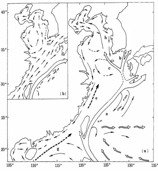
Guan (1994), Su (1998), Guo (2004) and Zheng et al. (2006) also gave the summer circulation of the Yellow Sea, respectively (Figure 1.3). All of these circulation patterns, in accordance with each other in essence, demonstrated the southward coastal current in the western Yellow Sea, only with some individual different detailed characteristics in the southern or the central parts. Most of the above researches were just on the basis of the hydrological datasets, since directly measurement in this area was restricted.

Beardsley et al. (1992) analyzed eight Satellite Tracking drifters released at 10 m depth, indicated there is a basin-scale cyclonic circulation in the upper layer of the Yellow Sea. The western Yellow Sea Coastal Current was still inferred to flow southward all the year round, associated with the cyclonic circulation. In later studies, the surface satellite-tracked trajectory data (Pang et al., 2004) and the current data of ADCPs (Acoustic Doppler Current Profilers) (Tang et al., 2004) implied that an anti-cyclonic circulation exists in the central part of Yellow Sea. The main focuses of these reports were the density current in the cold-water region rather than the coastal currents.

With the rapid development of computer technology, numerical modeling has been used widely to investigate the circulation in the Yellow Sea since the early 1980s, because of the lacks of the direct measurements. Lie (1999) concluded the numerical simulation in the Yellow Sea in detail.

The early numerical studies of Yellow Sea were restricted to the barotropic models for simplification, adopting the uniform wind system (Choi, 1982; Park,

(28)

1986b; An, 1987; Le et al., 1993; Zhu and Fang, 1994; Hsueh and Yuan, 1997). In summertime, the weak southerly wind and the strong surface heat flux result in the strongly stratified water in the most regions of Yellow Sea. While, the water is vertical mixed or weak stratification in the shallow coastal region because of the strong tidal mixing (Lie, 1989). Consequently, the early simulation results could not represent the summer circulation of Yellow Sea satisfactorily.

Later, the more exhaustive baroclinic models, considering the realistic wind forcing, surface heat flux, river discharge or tides, were used to investigate the response of the circulation in the Yellow Sea.

Yanagi and Takahashi (1993) used a diagnostic model to study the seasonal variation of the circulation pattern in the Yellow Sea. They suggested, in summer, a cyclonic circulation is developed at the upper layer and an anti-cyclonic one at the lower layer, and the circulations are mainly induced by the topographic heat accumulation effect (Takahashi and Yanagi, 1995).

Lee (1996) investigated the Yellow Sea circulation using a free surface primitive ocean model combined with realistic surface wind and heat flux, hydrography and the natural bathymetry. The model results for summer show that an anti-cyclonic circulation is formed both in the surface and the middle layers of the eastern Yellow Sea, with a cyclonic circulation in the surface layer of the western part. Xu et al.

(2002) studied the baroclinic circulation using the Modular Ocean Model (MOM2) with an ideal cylinder depth. Their results support the conclusion of Yanagi and Takahashi (1993).

(29)

Naimie et al. (2001) and Xia et al. (2006) simulated the circulations with tides forcing from the open boundaries, suggested a cyclonic circulation encompasses the central of Yellow Sea. Actually, according to their simulation results, the current along eastern coasts of China flows northward. Since the short of observations, these northward currents in the shallow coastal region have not been paid attention in both of these reports.

Later, Yuan et al. (2008) discovered that the Subei coast current actually flows northward in summer time in response to the southerly wind forcing. This northward flow was consistent with the satellite tracking of algal patches movements during the green tide event (Ulva Prolifera bloom) off Qingdao in the summer of 2008 (Hu and He, 2008; Qiao et al., 2008; Hu et al., 2010). Furthermore, the trajectories of ARGOS surface drifters released in the southwestern Yellow Sea in the summer of 2009 have confirmed this northward Subei coast current (Li, 2010).

Obviously, these reports also implied that the significance of the Lagrangian viewpoint in this region.

Liu and Hu (2009) suggested that northward flows dominate over the entire southwestern coast of Yellow Sea in summer, by analyzing a currentmeter data from ADCP located in the center of the Lunan trough. However, the study assumed tacitly that the Subei coastal current and the Lunan trough circulation are highly correlated, the variability of which can be represented by the moored measurement at the center of the Lunan trough. The previous studies also seem to support such an assumption. Later, Wang et al. (2013) suggested the west coastal currents in the

(30)

Yellow Sea are actually independent current systems controlled by different dynamics, due to the strong topographic effects.

Overall, the current theoretical and simulation researches on the circulations of Yellow Sea in different seasons have fairly advanced and already been widely accepted. However, the research of shallow southwestern region still needs some evidences to suggest the reliability of result.

(31)

1.3 The tides and tidal currents in the Yellow Sea

Since Ogura (1933) firstly provided the co-tidal charts of the four major tidal components (M2, S2, O1, K1) in the Northwestern Pacific, including the Yellow Sea, the strong tides and tidal currents in this area have been investigated widely from field observation data, satellite altimetric sea level data and a series of numerical models.

Guo and Yanagi(1998) and Naimie et al. (2001) reveled a detail review on this subject.

According to the existing results, the Eulerian tidal residual current forms a basin-scale cyclonic circulation in the central of the Yellow Sea, while it flows northward along the Subei coast as a part of an anti-cyclonic gyre. It has been suggested that the large tidal amplitudes over the sloping bottom around the Yangtze Bank, which lies between the basin scale cyclonic circulation and the anticyclonic gyre, produce strong southeastward residual currents.

In particular, the weak southerly wind and surface heating allow strong thermal stratification in summer leading to a significant sub-surface intensification of this southeastward tidal residual current (Lee and Beardsley, 1999), which could play an important role on the regional circulation. As mentioned above, previous studies revealed a cyclonic baroclinic circulation associated with the strong thermal fronts in the central of the Yellow Sea, roughly along the 40-50 m isobaths. The southeastward Eulerian tide-induced residual current is thought to strengthen this cyclonic circulation in the central part of the Yellow Sea in summer time (Xia et al.,

(32)

2006).

In all, the circulation in the Yellow Sea has been researched as early as 30s of the 20th Century (Uda, 1934; 1936). However, the basin geometry, the complex and shallow topography, the strong tides and the variable meteorology condition cause that the circulations in this area are extremely complex and difficult to model and predict. Due to the limited direct current measurements that have been obtained, the understanding of the circulation in the southwestern Yellow Sea is still primitive.

Furthermore, comparing with the Eulerian framework, the Lagrangian phenomena of the circulation has not been widely examined in this area. Therefore, It is more than necessary to check the Lagrangian framework of the circulation in the Yellow Sea.

(33)

In this thesis, the Lagrangian phenomena of the summer circulation in the Yellow Sea are studied on the basis of a series of high-resolution numerical experiments. The thesis consists of the following contents:

In Chapter 1, a general introduction on the circulation and the hydrological characteristics of the Yellow Sea has been reviewed.

In Chapter 2, the difference between the Lagrangian trajectories and Eulerian residual velocity fields in the southwestern Yellow Sea are investigated using a high-resolution circulation model.

In Chapter 3, the seasonal migration of the YSCBW and its controlling factors are studied on the basis of a series of high-resolution numerical experiments.

The last Chapter outlines our conclusions and outlooks, summarizes this study, and proposes the points that need to be developed in the further work.

(34)

Figure 1.1. Topography in the Bohai Sea, the Yellow Sea and the East China Sea.

Contour interval is 10 m.

(35)

Figure 1.2. Observed T-S diagrams of KODC dataset over 20 years from 1991 to 2010: (a) in February, (b) in August. Vertical connections between T/S points are

omitted.

YSWC water

PYSBCW

YSWC water YSBCW

CDW

(36)

Figure 1.3. Schematic representations of the circulation systems of the China Seas from Guan (1994) during winter (a) and summer (b) times, respectively.

(37)

Chapter 2 Difference between the Lagrangian Trajectories and Eulerian Residual Velocity Fields in the Southwestern Yellow Sea

Major part of this chapter has been published with open access at Springerlink.com, which entitled "Difference between the Lagrangian trajectories and Eulerian residual velocity fields in the southwestern Yellow Sea" (ID: ODYN-D-12-00103).

(38)

2.1 Introduction

As mentioned in the previous chapter, the Eulerian frameworks rather than the Lagrangian viewpoints are general widely used to explain the mass transport and circulation in the Yellow Sea. The straightforward definition of the Eulerian residual current is the averaged velocities at a fixed location over multiple tidal periods (Abbott, 1960).

However, the Eulerian residual currents do not always represent the net movement of the water parcel, especially in the shallow regions. As was first theoretically pointed out by Longuet-Higgins (1969), the velocity of the water parcel is controlled not only by the mean velocity at that point (Eulerian residual velocity) but also by the Stokes drift velocity. There are extra-dispersion terms in the inter-tidal transport equation (Fischer et al. 1979). In short, the Lagrangian trajectories do not necessarily follow the Eulerian residual velocity field in the presence of oscillatory tidal motion.

For instance, instead of following the southeastward Eulerian residual current, the ARGOS surface drifters released in the southwestern Yellow Sea in the summer of 2009 (Li, 2010), flowed northeastward and meandered through it (Figure 2.2). In other words, the Eulerian residual current flows southeastward over the sloping bottom around the Yangtze Bank, while the Lagrangian drifters extend northeastward, which could be a particular example of the above principle.

Some previous reports have demonstrated, both quantitatively and qualitatively, the differences between the tidal-induced only Lagrangian and the Eulerian residual

(39)

velocities in an idealized narrow bay (Ianniello, 1977; Jiang and Feng, 2011) and Bohai Sea (Breton and Salomon, 1995; Wei et al., 2004). Only a few researches (Feng, 1990; Delhez, 1996) have directly pointed out the accuracy of the Lagrangian residual current in representing the long-term transport in the light of the tides, atmospheric forcing and density-driven currents.

In the present study, we have used a numerical model to investigate the Lagrangian trajectories and the Eulerian residual velocity in response to tidal and wind forces in the southwestern Yellow Sea. This model could have practical applications, such as predicting green-tide events, which have occurred frequently on the beach of Qingdao city during recent summers. The data and model are described in the following section. The model validation and results of the numerical experiments are presented in Section 2.3. In Section 2.4 we consider the effects of using synoptic winds instead of climatological wind stress in the simulations. The last section outlines our conclusions.

(40)

2.2 Data and Model

The Princeton Ocean Model (POM) is applied to study the difference between the Lagrangian trajectories and the Eulerian residual velocity in the southwestern Yellow Sea. The model domain and topography are shown in Figure 2.1. The model covers the domain of (28°N-41°N, 117°E-128°E), with a horizontal resolution of 1/12°×1/12°. There are 16 vertical levels with sigma coordinates 0.000, −0.003,

−0.006, −0.013, −0.025, −0.050, −0.100, −0.200, −0.300, −0.400, −0.500, −0.600,

−0.700, −0.800, −0.900 and -1.00 from surface to bottom. The topography is averaged from 1′×1′ data of the Coastal and Ocean Dynamics Studies Laboratory of Sungkyunkwan University (Choi et al., 2002). Two modifications, setting the maximum water depth to 140 m and the minimum water depth to 10 m, are made to the original topography data to relax the CFL condition and to reduce possible errors in the finite-difference of the baroclinic pressure gradient over steep topography with a vertical sigma coordinate grid (Haney, 1991; Chen et al., 1995a, b).

Tidal forces including M2, S2, K1 and O1 are considered on the open boundary by using a fixed radiation condition for the depth-averaged velocity. The tidal amplitudes and phases are taken from the global 0.25°×0.25° TPX0.6 tide model (Gary et al., 1994). The tidal forcing is ramped up to full amplitude within the first two tidal periods to minimize starting transients. The time-mean Japanese 25-year re-analysis (JRA-25) wind stresses from 1983 to 1994 are considered as the climatology. The long-term daily-mean values are horizontally interpolated to force the numerical model. The model is integrated for two months from May to June

(41)

considering the weak wind effects. The initial and boundary conditions are determined from a 1/4°×1/5° Western North Pacific Ocean Model (Hirose, 2011), which are also 12 years averaged values during the same period with the wind stresses.

The sea surface temperature and salinity are relaxed to the climatology obtained from the same large-scale model instead of surface heat and salinity flux conditions.

Numerical experiments performed in this study are shown in Table 2.1. The first experiment TQ is conducted using only tidal forcing, whereas WQ uses only climatological wind forcing. The third experiment called WTQ includes both tidal forcing and climatological wind forcing. In all cases, the superscript Q means that the bottom friction term is given by the nonlinear quadratic parameterization:

(2.1)

where u is the near bottom velocity vector. The drag coefficient CD is 0.001 in the Bohai Sea, while it is 0.0016 in the other areas (Wan et al., 1998). The comparison of these three numerical experimental results will indicate the primary driving force of Lagrangian currents in the southwestern Yellow Sea. As the bottom friction has strong effects on the regional circulation (Jiang and Feng, 2011), additional experiments TL, WL and WTL are designed to check the effects of the bottom friction.

The superscript L means that the linear bottom friction scheme is used.

(2.2)

Apart from the bottom friction scheme, the experiments TL, WL and WTL assume the same conditions as TQ, WQ and WTQ, respectively. After some sensitivity experiments to match the nonlinear cases in terms of kinetic energy, we chose the

(42)

linear drag coefficients Γ_L to be 0.0005 in the Bohai Sea and 0.0008 in the other areas.

The movement of the upper layer water parcel in the southwestern Yellow Sea is studied by modeling the trajectories of the modeled drifters, which are deemed to be Lagrangian tracers. A hundred modeled drifters are released at a depth of 15 m along the 33.80°N section (Figure 2.1). In each experiment the positions of the drifters are calculated every 2 computational hours after the model has been running for 15 simulated days.

The trajectories are calculated by the fourth-order Runge-Kutta scheme according to Press et al. (1992), which is presented as follow.

(2.3)

(2.4)

(2.5) (2.6)

(2.7)

where 𝑥_! is the previous position, 𝑥_!!! is the predicted position of the drifter after one time step (∆𝑡) and u is the velocity. This method is reasonably simple and robust and is a good general candidate for numerical solution of differential equations when combined with an intelligent adaptive step-size routine. Since the model

(43)

velocities are assigned in the horizontal resolution of 1/12°×1/12°, the velocities and the topographies are interpolated to the position of the drifter in each time step (∆𝑡) by the bilinear interpolation method.

(44)

2.3 Results

2.3.1 Water mass distribution

The simulated temperature structures along the vertical sections at 33°N and 35°N in June (Figure 2.3) are compared with the climatological temperature obtained from the U.S. Navy’s Generalized Digital Environmental Model (GDEM). The GDEM version 3.0 is a global monthly mean three-dimensional temperature and salinity data set with a horizontal resolution of 1/4° over the world oceans and with 78 vertical levels (0-6600 m). This data set has been built on the U.S. Navy’s Master Oceanographic Observation Data Set (MOODS) with 8 million profiles.

Roughly, the basic features of the summer stratification and water mass distributions are represented well by the baseline experiment WTQ, suggesting that the simulated circulation reproduces the basic characteristics of the summer circulation in this region.

Both the simulated and observed temperatures are vertically uniform at the coastal area of the 33°N section (Figure 2.3a and Figure 2.3b), indicating that vertical mixing is strong in this shallow area due to tidal motion (Zhao et al., 1994; Xia et al., 2006). In the central Yellow Sea, a vertical temperature gradient starts to form, characterizing the seasonal thermocline, separating the water column into upper and lower layers. The upper part of the seasonal thermocline is elevated toward the sea surface while the lower part of it forms a strong front at a depth of roughly 15-20 m.

Along the vertical section of 35°N in both the simulated and observed

(45)

temperatures (Figure 2.4a and Figure 2.4b), the western core of the Yellow Sea Cold Water Mass is identified at a depth of 40-50 m over the slope on the western flank of the Yellow Sea trough. The intensity of the cold core is weaker than the observation due to the influence of the initial and surface conditions, which are not exactly climatological ones, after merely 2 months of model integration.

The pattern of the horizontal isohaline and the low salinity tongue of the Yangtze River diluted water also generally agree with climatological salinity from GDEM data set (not shown here). All of the characters, including the thermocline and the position of the surface and subsurface water masses, are simulated well by the experiment WTQ, implying that the present model has captured the essential dynamics of the current systems.

2.3.2 Verification of the simulated tides

To verify the simulated tides, only tidal forcing with homogenous water are tested in the model at first, and the temperature and salinity are set to 21°C and 33.5 PSU, respectively. In this case, the model approaches steady state after about 5 days.

After 15 days, harmonic constants are obtained by harmonic analysis. The co-tidal charts of the M2, S2, K1 and O1 tides generated from the model are shown in Figure 2.5. These structures basically agree with the previous studies (Fang, 1986; Yanagi et al., 1997; Guo and Yanagi, 1998; Kang et al., 1998; Lee and Beardsley, 1999; Bao et al., 2000; Fang et al., 2004). All of the semi-diurnal amphidromic points (M2 and S2 tides) and the diurnal amphidromic points (K1 and O1 tides) in the southwestern

(46)

Yellow Sea are reproduced successfully.

Forasmuch as the limitation of tidal observations, only M2 tidal harmonic constants from the model are compared with observed values of 63 sites as shown in Figure 2.1. The observed data comes from Wan et al. (1998) and Zhang et al. (2005), and the model values are used after interpolation. The standard deviations between the simulated and observed M2 tidal amplitude and phase for all sites are 9.3 cm and 12.0 degree (Figure 2.6). The results show that the simulated M2 tide agrees the observations well. The results with climatological stratification (not shown here) are essentially the same as those with homogenous water.

2.3.3 Eulerian residual velocity fields

The simulated tide-induced residual current at 15 m during June in TQ (Figure 2.7a) shows a basin-scale cyclonic circulation in the Yellow Sea. The result is similar to those of existing studies (Zhao et al., 1993; Lee and Beardsley, 1999; Xia et al., 2006). Three obvious characteristics of the Eulerian tide-induced residual current have been reproduced. The first feature is the strong northward current around the southwest of Korea with a maximum speed of 10 cm/s. The second feature is the northward flow along the Subei coast (water depth less than 15 m, can not be illustrated in Figure 2.7a), forming an anticyclonic gyre in the area. The third feature is the strong long-range southeastward current with a speed of ~5 cm/s over the sloping bottom around the Yangtze Bank, between the basin-scale cyclonic circulation and the anticyclonic gyre. Generally, the tides and tidal currents

(47)

produced by the model agree well with previous studies.

By including wind forcing, a more realistic circulation is generated in experiment WTQ. As shown in Figure 2.7b, the circulation at a depth of 15 m in June is a cyclonic circulation that encompasses the entire deep basin. Along the Korean coast, the northward flow is strong; on the other hand, in the western and central parts of the Yellow Sea, the current flows southward and is much broader and weaker. In particular, along the Subei coast, the northward current is enhanced by tidal rectification (can not be presented in Figure 2.7b). With the strong southeastward current over the sloping bottom around the Yangtze Bank, an anticyclonic gyre is formed next to the western limb of the cyclonic current. This result is similar to the model result of Naimie et al. (2001) and the analysis of observations in Liu (2006). The realistic features of the present model allow us to study the dynamics of the Lagrangian trajectories in the southwestern Yellow Sea.

2.3.4 Lagrangian trajectories

The Lagrangian phenomena are studied by using the trajectories of modeled drifters. Table 2.1 shows the mean meridional displacement of the modeled drifter movements after 45 days in each experiment. A positive value means northward movement whereas a negative value means southward movement. It should be pointed out that the thermohaline conditions and wind stress are based on climatological fields. The simulated trajectories of the modeled drifters represent a climatological Lagrangian circulation field while the observations are in the summer

(48)

of a particular year. Therefore, more attention should be paid to the differences between experimental results instead of being concerned with the accurate reproduction of observed trajectories.

The modeled drifters in TQ (only tidal forcing), released at the northeastern flank of the Yangtze Bank, flow southeastward at high speed (Figure 2.9a). The other drifters released at the shallow western area flow northward at a lower speed. The mean meridional displacement of all the modeled drifters is about −59.28 km (Table 2.1), and the patterns of the trajectories look like the tendency of the streamlines as shown in Figure 2.8a. However, it is actually distinct from the mean meridional displacement of −73.24 km for trajectories that are directly driven by the Eulerian tide-indeuced residual current (not shown here). The dissimilarity between the two sets of trajectories indicates that the Lagrangian and the Eulerian residual velocities are different, in agreement with previous studies (Longuet-Higgins, 1969; Ianniello, 1977; Jiang and Feng, 2011).

In comparison, in experiment WQ (only climatological wind forcing) almost all these modeled drifters released at the northeastern flank of Yangtze Bank flow northeastward (Figure 2.9b). The mean meridional displacement of these modeled drifters exceeds +110 km (Table 2.1).

In experiment WTQ (including both tidal and climatological wind forcing), the modeled drifters move in the similar directions as in WQ. We especially noticed a difference for the modeled drifters deployed at the northeastern flank of Yangtze Bank: these modeled drifters do not flow directly northeast but begin by moving

(49)

southeast due to the effects of the strong long-range southeastward Eulerian residual current over the sloping bottom around the Yangtze Bank, as illustrated in the small box of Figure 2.9c. However, the drifters easily drop out of the Eulerian residual current and move further northeastward. This indicates that the Stokes drift velocity of tidal motion is comparable in magnitude to the Lagrangian residual velocity, and eclipses the Eulerian residual velocity. In the other words, the Lagrangian trajectories (path lines) do not follow the streamlines of the Eulerian residual velocities (Figure 2.8b). The weighted center of the modeled drifters moves northward by about 97.33 km from the initial latitude (Figure 2.9c). The pattern of these trajectories corresponds with observations of the ARGOS surface drifters released in the southwestern Yellow Sea in the summer season of 2009 (Li, 2010).

To examine the effects of wind and tide on the Lagrangian trajectories respectively, the simple average of the velocity field snapshots of WQ and TQ are calculated. The simple linear combination of WQ and TQ (Figure 2.9d) results in a mean meridional displacement of only +52.52 km (Table 2.1), which is much less than that in WTQ. The tidal effect in WTQ is obviously weaker than what is expected from the linear combination. Furthermore, the experiments in which the modeled drifters are released at surface layer also arrive at the same conclusion (not shown here). Thus, the wind stress is the dominant factor determining the Lagrangian trajectories in the upper layers of the southwestern Yellow Sea in summer, which could explain the transport of large numbers of green tide patches from Subei to Qingdao during recent summers.

(50)

To further understand the dynamics of these Lagrangian phenomena, the effect of bottom friction has been examined by considering the linear bottom friction scheme. TL, WL and WTL have the same conditions as TQ, WQ and WTQ, respectively, except for the use of the linear bottom friction scheme. As shown in Figure 2.10a, the results of WTL resemble those of WTQ. The mean meridional displacement of the modeled drifters in WTL is about +98.85 km (Table 2.1). In contrast, the linear combination of WL and TL (Figure 2.10b) results in a mean meridional displacement of +92.30 km (Table 2.1), which is relatively similar to WTL, in contrast with the nonlinear cases. These results suggest that, in this region, the Lagrangian trajectories can be simply determined by linear dynamics without a quadratic friction term. In other words, the nonlinearity of the bottom friction plays an important role for the weaker influence of the tide-induced residual currents on Lagrangian trajectories in the southwestern Yellow Sea.

In general, bottom friction is an important sink of momentum and energy in the ocean, especially for shallow areas where the surface and bottom boundary layers easily affect and interact each other. The bottom momentum fluxes (hereafter BMFs) in POM are represented by

𝜌× wu −1 , wv −1 = −ρ×C_! uu (2.8)

where u and C_! have same meanings as in equation (2.1), and –1 presents momentum fluxes at bottom. The density of seawater ρ is 1.025 kg/m³. In the linear bottom friction parameterization approach mentioned above (equation (2.2)), the BMFs are

(51)

𝜌× wu −1 , wv −1 =−ρ×Γ_!u (2.9)

Equations (2.8) and (2.9) are similar if we assume that Γ_L=CDU, where U is the typical speed of linear bottom friction. The difference between the two expressions is that U is a constant (0.5 m/s), whereas, |u| is time- and space-dependent.

The magnitudes of the area-averaged BMFs are shown in Table 2.1. In accordance with the results described above, the BMFs of WTL and WTQ are very similar (12.3×10^-3 N/m²and 12.7×10^-3 N/m², respectively) which means WTL can reproduce WTQ by choosing the appropriate value of U. However, the BMF in TL

(5.8×10^-3 N/m²) is 28.40% weaker than that of TQ (8.1×10^-3 N/m²) in the shallow area, whereas it is considerably enhanced in WL (8.6×10^-3 N/m²) in contrast to that of WQ

(1.7×10^-3 N/m²).

As mentioned above, the BMFs given by quadratic and linear relations are approached, when the magnitude of current becomes close to the speed of linear bottom friction (0.5 m/s). If the magnitude of current over the speed of linear bottom friction, the quadratic function curve to define BMFs should be greater than linear relation. On the contrary, it is opposite if the current weaker than the speed of linear bottom friction. In the southwestern Yellow Sea, the tidal currents are usually stronger than the typical speed of linear bottom friction (0.5 m/s). Conversely, the wind-driven currents in this area are normally weaker than 0.5 m/s, meaning that the BMFs of wind effects given by the quadratic relation are weaker than those given by the linear relation.

Thus, it indicates that the quadratic bottom topography shear leads to strong

(52)

steering effects on the regional circulation in summer. The larger BMFs in the experiment TQ utilizing the quadratic bottom friction scheme lead to a weaker tidal effect than the one in TL. The wind effect, however, shows the opposite behavior:

the BMFs in experiment WQ,which uses the quadratic bottom friction scheme, are much smaller than those in WL, resulting in a stronger wind effect.

(53)

2.4 Effects of Synoptic Forcing

The wind forcing employed in previous sections was climatological wind stress from May to June. The realistic wind with a high frequency (synoptic variability) might have an impact on the behavior of the upper layer drifters. To examine the effects of synoptic winds and to enhance the generality of the results described in the previous section, additional experiments were carried out, in which the JRA-25 6-hourly wind stresses from May to June in 2009 and 2010 were adopted instead of climatology.

For comparison, in the experiment forced by the tidal forcing and the wind stresses from May to June in 2009, the pattern of the modeled drifter trajectories successfully reproduces observation of the ARGOS surface drifters (Figure 2.11).

Since the wind stress from May to June is feebler than that of observed period, then the final weighted center of these drifters arrives at 35.62°N, where is slightly south off that of observation. The characters of the ARGOS surface drifters trajectories are simulated well by this experiment, showing once again that the present model has caught up the realistic features of the regional circulation.

The southerly wind in June of 2009 has almost same magnitude comparing with the climatological monthly mean one. Their difference is essentially the existence of high-frequency (synoptic) component. Combining with above results, the following conclusion can be drawn: the high frequency realistic wind could enhance the wind effects on the behavior of the upper layer drifters. While, the monthly mean

(54)

climatological one as shown in Figure 2.12. The wind effects on Lagrangian trajectories would be minimal in 2010. The experiments forced by wind stress of 2010 should be representative, thus only which are used to check the effects of synoptic winds because of paper length. The character R is used to indicate the use of realistic wind forcing in the experiments.

The patterns of the Lagrangian trajectories are essentially the same as those in the climatological experiments. In RTQ (Figure 2.13a), the modeled drifters released at the northeastern flank of the Yangtze Bank flow northeastward with a mean meridional displacement of +61.74 km (Table 2.2). In this case, the northeastward movement of artificial drifters is suppressed due to the weaker southerly monsoon in summer season of 2010. In the linear combination of RQ (only forced by realistic wind) and TQ (only forced by tidal forcing) the mean meridional displacement is +16.22 km (Figure 2.13b). So, even with the realistic weak wind forcing of 2010, the influence of the Eulerian tide-induced residual currents on the Lagrangian trajectories is still weaker than the wind effect.

RTL, which uses the linear bottom friction scheme, reproduces the results RTQ

(Figure 2.13c) with a mean meridional displacement of +66.41 km. The result of a simple linear combination of TL and RL (Figure 2.13d) is almost the same as the simulation of RTL, giving a mean meridional displacement of +62.38 km (Table 2.2).

In conformity with the climatological cases, the nonlinearity of the bottom friction leads to a weaker influence of the Eulerian tide-induced residual currents on the Lagrangian trajectories in the upper layer of the southwestern Yellow Sea.

(55)

In a normal year, the southerly wind from May to June is stronger than that of 2010. Thus, the wind effect is expected to be much stronger and the effect of the Eulerian tide-induced residual current on Lagrangian trajectories may be relatively minor in any other summer. Therefore, the experiments using the realistic wind stress of 2010 might indicate the minimum size of the wind effect, and it still shows that the wind effects are dominated for the movements of Lagrangian drifters in the upper layer. Thus, considering the individual characteristics of wind forcing in 2009 and 2010, the conclusions are considered to be general for this region.