On Weak Approximation of Stochastic Differential Equations with Discontinuous Drift Coefficient (Mathematical Economics)

(1)

On

Weak

Approximation

of

Stochastic

Differential

Equations

with

Discontinuous

Drift

Coefficient

1

Arturo Kohatsu-Higa

DepartmentofMathematical Sciences

Ritsumeikan University

1-1-1 Nojihigashi,Kusatsu, Shiga, 525-8577, Japan.

Antoine Lejay

Project-teamTOSCA, Institut

\’Elie

CartanNancy

(Nancy-Universit\’e,CNRS, INRIA)

BP 239, F-54506 Vandoeuvre-les-Nancy, France.

Kazuhiro Yasuda

Faculty ofScienceandEngineering

Hosei University

3-7-2, Kajino-cho, Koganei-shi,Tokyo, 184-8584, Japan.

Abstract

Inthispaper,weakapproximationsofmulti-dimensional stochastic differential

equa-tionswithdiscontinuousdrift coefficientsareconsidered. Hereastheapproximated

pro-cess, theEuler-Maruyama approximationof SDEs withapproximateddriftcoefficients

isused, andweprovidearateofweakconvergenceof them. Finallywepresentarate

ofweakconvergenceof the Euler-Maruyamaapproximationof the original SDEs with

constantdiffusion coefficients.

1 Introduction

Inmathematical finance,

one

describes assetprice processes

as

the solutionto the following

stochasticdifferential equations(SDEs):

$dX_{t}=b(t,X_{t})dt+\sigma(t,X_{t})dW_{t}$

.

(1.1)

where $b$ and $\sigma$

are

certain fimctions and $W_{t}$ is

a

Brownian motion. Then

we

consider

a

flmction $f$, which represents

a

payoff mnction in financial derivatives, and

one

write its

associatedoptionprice

as

the

expectation

$E[f(X_{T})]$, where $T$is

a

maturity

ofthe option

and

$X_{T}$ isthe assetprice at$T$

.

Notethat

we are

using the

interpretation

oftheexpectation using

a

financial situation, but, ofcourse, it isalso important inmanyother fieldsand applications.

Itis

rare

theoccasion when

one

isabletocalculate theprevious expectationanalytically.

Therefore inorder toobtainitsvalue,

one

resortsto computer simulations andtriestoobtain

lThispaperisanabbreviated and preliminaryversionof A. Kohatsu-Higa, A. Lejay and K. Yasuda[5]. If

(2)

anapproximated value. Inpractice,twokinds ofapproximations

are

neededtosimulate this

expectation. One is

an

approximation of the SDEs (1.1) and the other is

an

approximation

of the expectation. For the latter,

one can

typically

use

the Monte-Carlo method, which is

based

on

law of large numbers

in

probability theory. On the otherhand, forthe former, the

Euler-Mamyama approximation is often used. The Euler-Maruyamaapproximation

can

be

described

as

follows: For simplicity,

we

split theinterval $[0, T]$ equallyin$n$subintervalsand

let the length of eachtime subinterval$\Delta t$be equalto $\frac{T}{n}$,

$\overline{X}_{0}=x$, $\overline{X_{i+1}}=\overline{X_{i}}+b(i\Delta t,\overline{X_{i}})\Delta t+\sigma(i\Delta t,\overline{X}_{i})\sqrt{\Delta t}\xi_{i}$,

where the random variables $\xi_{i},$ $i=0,1,$$\cdots,n-1$,

are

independent ofeach other and

are

distributed according to

a

$N(O,I_{d})$ law, where $0$ is the d-dimensional

zero

vector and $I_{d}$ is

$d\cross d$-unit matrix. When

we

approximate stochastic

processes, one

needs

a

criteria in order

to determine the quality ofthe approximation. One mainly

uses

the following two criteria

(strong

error

and weakerror): the definition of

an

approximation with strong

error

of order

$\gamma>0$ is that there

exists

a

positiveconstant$C$,which doesnotdepend

on

$\Delta t$, such that

$E[|X_{T}-\overline{X}_{n}|]\leq C\Delta t^{\gamma}$

.

Under enough regularityfor coefficients $b$ and$\sigma$, the strong $elTor$has the order 1/2 for the

aboveEuler-Maruyama approximation. For

more

details, readers

can

referExercise 9.6.3 in

Kloeden and Platen[4]. Thedefinition ofweak

error

withorder$\gamma>0$is that forallffinctions

$f$in

a

certain class, there exists

a

positive constant $C$, which does not depend

on

$\Delta t$, such

that

$|E[f(X_{T})]-E[f(\overline{X}_{n})]|\leq C\Delta t^{\gamma}$

.

Here under enoughregularity

on

the coefficients $\sigma$and $b$ and

on

$f$,

we

have the weak

error

withorder 1 for the Euler-Mamyama approximation.

The

purpose

ofthis paper is to treat

an

SDE with discontinuous drift coefficients and

obtain

an

order ofweak

error

foritsapproximation. Precisely speaking,

we

consider

an

SDE

with

an

approximateddrift coefficient $b_{\epsilon}$,which isapproximatedusingthe Euler-Maruyama

approximation. Then,

one uses

theapproximatedprocess

as

theapproximation ofthe original

SDEs. Then

we

estimate

an

order of the weak

error

between the original SDEs and the

approximated process. Inthe latterpart ofthis article,

we

deal with

an

SDE with constant

diffusion coefficients and obtain

an

order of the weak elTor between the SDEs and their

approximated

process

towhich theEuler-Mamyamaapproximationis directly applied.

SDEs with discontinuous drift coefficients

are

of

course

used in various fields. For

in-stant, in mathematical finance, if

one

wants to model

a

stock price process whose trend

dramatically changeswhen

a

factor

goes

down

a

threshold value. Inthis case, the drift

can

be modeled

as

taking two values specified by

some

indicator hnction. This kind of SDE

also

appears

in

some

control problems.

Weak

error

of SDEs with discontinuous coefficients(notonly driftcoefficients, but also

(3)

their

papers,

they only proved weak

convergence

ofthe Euler-Mamyama

approximation,

not

mentioned

an

order ofthe weak

convergence.

Andalsostrong

error

and therate

are

studied

in Przybylowicz [10] for SDEs with

some

type of discontinuous coefficients. Note thatin

this

paper,

the diffusion coefficients of

our

SDEs have enoughregularity.

This

paper

is organized

as

follows:

Some

notations

and

assumptions

are

given in

Sec-tion

2.

Weprovide

our

main result

on a

rate ofweak

errors

under SDEs with discontinuous

driftand nonlineardiffusion coefficient in Section3, andalso give results underconstant

dif-ffision coefficientsin Section 4. Finally

we

give

some

numerical resultsin Section 5. Proofs

oftheorems and

so

on

below

can

be found inKohatsu-Higa, LejayandYasuda[5].

2 Notations

and

Hypotheses

Let$d\in \mathbb{N}$

.

The

space

ofcontinuousffinctions that

are

slowly increasingis denotedby$C_{Sl}(\mathbb{R}^{d})$

.

Afimction$f$in$C_{Sl}(\mathbb{R}^{d})$is such that forevery$k>0$,

$\lim_{|x|arrow\infty}|f(x)|e^{-k|x|^{2}}=0$

.

Fix $T>0$

.

Let$H$be the set $[0, T)\cross \mathbb{R}^{d}$and$\overline{H}=[0, T]\cross \mathbb{R}^{d}$

.

Let $\sigma$ be

a

measurable fimction

on

$[0, T]\cross \mathbb{R}^{d}$ with values in the

space

of symmetric

$d\cross d$-matrices. We set$a=\sigma\sigma^{*}$ and

assume

that

there exist

some

positiveconstants$\Lambda$ and$\lambda(\Lambda\geq\lambda>0)$

(Hl)

suchthat$\lambda|\xi|^{2}\leq\xi^{*}a(t,x)\xi\leq\Lambda|\xi|^{2}$, for all $(t,x)\in\overline{H}$, andall$\xi\in \mathbb{R}^{d}$,

$\sigma$isuniformlycontinuous

on

H. (H2)

Remark2.1 Note that (Hl)givesa lower andupperboundon the eigenvalues

_of

$a$, which

are

_from

the veryconstruction equalto the eigenvalues

_of

$\sigma$ (wehave chosen $\sigma$ to be

sym-metric)

_for

which(Hl)holds with $\lambda$and$\Lambda$replacedby $\sqrt{\lambda}$and $\sqrt{\Lambda}$

.

Let

us

alsoconsider

a

measurable fimction$b$ ffom$[0, T]\cross \mathbb{R}^{d}$to$\mathbb{R}^{d}$such that

$|b(t,x)|\leq\Lambda$ forall$(t,x)\in H.$ (H3)

From

now

on,

we

always

assume

(Hl), (H2)and(H3)for$b$ and$\sigma$

.

Now,

we

give

some

notations.

Fix $\alpha>0$

.

Let $H^{\alpha}(\mathbb{R}^{d})$ be the

space

ofcontinuous,

bounded fimctionswith continuous,bounded derivatives uptoorder$\lfloor\alpha\rfloor$and such that$\partial_{x}^{\lfloor\alpha\rfloor}f$is

$(\alpha-\lfloor\alpha\rfloor)$-H\"oldercontinuous. Let$H^{\alpha/2,\alpha}(\overline{H})$be thesetofcontinuous fimctions with continuous

derivatives$\partial_{t}^{r}\partial_{x}^{s}u$ for all $2r+s<\alpha$andsuchthat

$||u||_{H^{\alpha\prime 2.\alpha}}= \sum_{2r+s\leq\lfloor\alpha\rfloor}\sup_{(t,x)\in\overline{H}}|\partial_{t}^{r}\partial_{x}^{s}u(t,x)|+\sum_{2r+s--\lfloor\alpha\rfloor}\sup_{(t,x),(ty)\in\overline{H}}\frac{|\partial_{t}^{r}\partial_{x}^{s}u(t,x)-\partial_{t}^{r}\partial_{x}^{s}u(t,y)|}{|x-y|^{\alpha-\lfloor\alpha\rfloor}}$

$+$$\sup_{0<\alpha-2r-s<2(t,x),(v,x)\in\overline{H}}\frac{|\partial_{t}^{r}\partial_{x}^{s}u(t,x)-\partial_{t}^{r}\partial_{x}^{s}u(v,x)|}{|t-v|^{(\alpha-2r-s)/2}}$$\sum$

(4)

3 Main Theorems

Let$\sigma$and $b$ satisfy $(H1)-(H3)$

.

These conditions

are

sufficient to

ensure

the existenceof

a

uniqueweaksolution$(X, (\mathcal{F}_{t}’)_{t\geq 0},\mathbb{P}_{x})$to

$X_{t}=x+ \int_{0}^{t}\sigma(s,X_{s})dB_{s}+\int_{0}^{t}b(s,X_{s})ds$ (3.1)

for

a

Brownianmotion$B$

.

Remark3.1 $IfX_{t}=x+ \int_{0}^{t}\sigma(s,X_{s})dB_{s}$hasastrongsolution,then(3.1) also admits astrong

solution (See Veretennikov [11]).

Let$b_{\epsilon}$ be

a

family of measurable

coefficients

on

$\overline{H}$

with $|b_{\epsilon}(t, x)|\leq\Lambda$ for $(t,x)\in\overline{H}$

.

Let

us

considerthe unique weak solution$(X^{\epsilon}, (F_{t})_{t\geq 0}, \mathbb{P}_{x})$to

$X_{t}^{\epsilon}=x+ \int_{0}^{t}\sigma(s,X_{s}^{\epsilon})W_{s}+\int_{0}^{t}b_{\epsilon}(s,X_{s}^{\epsilon})ds$

.

(3.2)

Since $b_{\epsilon}$ and$b$

are

bounded, thedistributionof$X^{\epsilon}$

may

be deduced ffomthe distribution

of$X$through

a

Girsanov transform.

For $T>0$, let$T$ _be_the_continuous_{solution of the Euler-Mamyama scheme of}_step _size

$T/n$

.

If$\phi(s)=\sup\{t\leq s|t=k/n$ for$k\in \mathbb{N}\}$,then

$T_{t}=x+ \int_{0}^{t}\sigma(\phi(s),z_{\phi(s)})dB_{s}+\int_{0}^{t}b_{\epsilon}(\phi(s),r_{\phi(s)})ds$

.

(3.3)

When$\sigma$and$b_{\epsilon}$belongto

an

appropiateclassofffinctions$\mathfrak{M}$(forexample$\mathfrak{M}=H^{\alpha/2,\alpha}(\overline{H})$

for

some

$\alpha>0$

or

$\mathfrak{M}=C_{b}^{1,3}(\overline{H}))$, and when_$f$belongs to

a

proper

class of ffinctions $S$ (for

example, $ff=H^{2+\alpha}(\mathbb{R}^{d})$

or

$S=C^{3}(\mathbb{R}^{d})\cap C_{Sl}(\mathbb{R}^{d}))$,

a

rate of weakconvergenceof the

Euler-Mamyamascheme$\mathscr{K}^{-}$

is known. This

means

thatthereexists

some

constant$C_{\epsilon}$such that

$| E[f(X_{T})]-E[f(\overline{X}_{T}^{\epsilon})]|\leq\frac{C_{\epsilon}}{n^{\delta}}$

.

Assumethat$C_{\epsilon}=O(\epsilon^{-\beta})$

.

Thisisin generalthe

case

when

one

choosesto

use a

regularization

$b_{\epsilon}$ of$b$byusingmollifiers.

Onthe otherhand,

as we

will show below inProposition 3.2 and Remarks 3.3 and 3.5,

one

has

$| E[f(X_{T})]-E[f(X_{T}^{\epsilon})]|\leq C’E[(\int_{0}^{T}|b(s, Y_{s})-b_{\epsilon}(s, Y_{s})|^{p}ds)^{q/p}]^{\iota/q}$ _(3.4)

for

some

appropriate values of$p$and$q$and positive constant$C’$

.

Assume that thequantity inthe right-hand side of(3.4)decreasesto$0$

as

$O(\epsilon^{\gamma})$.

(5)

Assume that$f$belongs to

some

appropriate class

offunctions

$\mathfrak{F}$, and

an

approximation

$b_{\epsilon}$

of

the

drift

$b$belongs to

some

class

offmctions

SEJt

in

a

way

such that

$|E[f(X_{T})]-E[f(X_{T}^{\epsilon})]|=O(\epsilon^{\gamma})$ (3.5)

and

$| E[f(X_{T}^{\epsilon})]-E[f(\overline{X}_{T}^{\epsilon})]|=O(\frac{1}{\epsilon^{\beta}n^{\delta}})$

.

(3.6)

Then

_for

$\epsilon=O(n^{-\delta/(\gamma+\beta)})$,

$| E[f(X_{T})]-E[f(\overline{X_{T}^{-}})]|\leq O(n^{-\kappa})where\kappa=\frac{\delta\gamma}{\gamma+\beta}$

.

Under the

assumptions

(3.5) and(3.6),

we

have the order$\kappa$of the weak

error among

the

SDEs (3.1) and the approximated

process

(3.3). Therefore, ffom

now

on,

_our

interest is

to

find

some

conditions that theassumptions(3.5) and(3.6)hold.

3.1 A

Perturbation Formula

Through Theorem

3.2

andthe remarksbelow,

we can

find

some

situations

where

Assump-tion(3.5)holds.

Let$X$be the solutionto (3.1) and$X^{\epsilon}$ be the solutionto (3.2).

Theorem3.2 For$\alpha>2$and_$p>2$such that _{$1/\alpha+1/p<1/2$}and$f\in C_{Sl}(\mathbb{R}^{d})$,

$|E[f(X_{T})]-E[f(X_{T}^{\epsilon})]|\leq C_{2}(\alpha,p, T)A_{T}(\epsilon)\sqrt{Var_{\mathbb{P}}(f(X_{T}))}$

with

$C_{2}( \alpha,p, T)=T^{1/2-1/p}\exp(T\Lambda^{2}\lambda^{-1}(\alpha-\frac{1}{2}+(1-\frac{2}{\alpha})\frac{\alpha(\frac{1}{2}+\frac{1}{p})-1}{\alpha(\frac{1}{2}-\frac{1}{p})-1}\Vert$ ,

$A_{T}( \epsilon)=E^{0}[\int_{0}^{T}|b_{\epsilon}(s, Y_{s})-b(s, Y_{s})|^{p}ds]^{1/p}$,

where$(Y, \mathbb{P}^{0})$isthe weak solution to $Y_{t}=x+ \int_{0}^{t}\sigma(s, Y_{s})dW_{s}$

for

some

Brownianmotion $W$

.

Remark

3.3

Let

us assume

that

an

upper Gaussianestimateholds

_for

the transition density

function

$p(t,x,y)$

of

$Y$

defined

by$Y_{t}=x+ \int_{0}^{t}\sigma(s, Y_{s})dW_{s}$

.

This

means

thatfor

some

constants

$C_{1}$ and$C_{2}$,

(6)

for

all$(t,x,y)\in \mathbb{R}_{+}\cross \mathbb{R}^{d}\cross \mathbb{R}^{d}$

.

Then

for

any _{$1<r,q\leq+\infty$}

satisf2

$ingd/2r+1/q<1$_, it

follows

that

$A_{T}( \epsilon)\leq C_{3}(\int_{0}^{T}(\int_{\mathbb{R}^{d}}|b(s,y)-b_{\epsilon}(s,y)|^{pq}dy)^{r/q}ds)^{1/rp}=C_{3}||b-b_{\epsilon}||_{L^{rp.qp}(H)}$_, where$C_{3}$ isacertainpositiveconstant$C_{3}$,

andfor

$r<+\infty$set

$||f \rceil|_{L^{r.q}(H)}=(\int_{0}^{T}(\int_{0}^{T}|f(s,x)|^{q}dx)^{r/q}ds)^{1/r}$

and alsoset$||J||_{L^{\infty,q}(H)}= \sup_{t\in[0,T]}||f(t, \cdot)||_{Lq}$.

Remark3.4 Such estimate (3.7) holds

_for

example $\iota f$the

diffusion

coefficient

_$a$ belongs to

$H^{\alpha/2,\alpha}(H)$

for

some

$\alpha>0$ (See

for

example Ladyzenskaja [7, \S IV. 13,

p.

377]).

Remark3.5 Even inabsence

_of

a Gaussian upperbounds, the$K’\gamma lov$estimate (Krylov [6]

orBass [1, Theorem 7.6.2, p. 114]$)$ couldalso be used with Hypothesis(Hl)inorderto get

anestimate

on

$A_{T}(\epsilon)$

.

In this

case

_$ofa$homogeneous

coefficient

$b$_,

from

theKrylovestimate,

we

have

$|A_{T}(\epsilon)|\leq C(\lambda, \Lambda)e^{T}||b-b_{\epsilon}||_{L^{dp}}$

.

Incase$ofa$time-inhomogeneouscoefficient, asimilarestimatecould be obtained buton the

bounded domaincaseand

one

should thenestimatetheexit time

_from

such domains.

3.2 Rates

of

Convergence of

the

Euler-Maruyama Approximation

with

Regular Enough

Coefficients

We

now

exhibit

some

situationswhere Assumption(3.6) holds, underthe weakest possible

assumptions

on

the regularity of the coefficients. Note that other results may hold (See

Theorem4.3 below).

3.2.1 Caseof$Hlder$continuous coefficients

The weak rate of

convergence

of the Euler scheme when the coefficients of the PDE

are

H\"older_continuous_{has been smdied by R.} _Mikulevicius _{and E. Platen}[9].

Theorem 3.6(R.Mikulevicius andE. Platen[9])

_Iffor

$\alpha\in(0,1)\cup(1,2)\cup(2,3),$ $b$anda

belongs to$H^{\alpha/2,\alpha}(\overline{H})$ and$f\in H^{2+\alpha}(\mathbb{R}^{d})$, then thereexists

a

constant$K$suchthat

$| E[f(X_{T})]-E[f(\overline{X}_{T})]|\leq\frac{K}{n^{E(\alpha)}}$

with

$E(\alpha)=\{\begin{array}{ll}\alpha/2 \iota f\alpha\in(0,1),1/(3-\alpha) \iota f\alpha\in(1,2),1 \iota f\alpha\in(2,3).\end{array}$

(7)

3.2.2 Case

ofsmooth coefficients

Theorem 3.6 requires the coefficientsto beH\"oldercontinuous. Of course, the

convergence

rate isbetter for smooth coefficients. But in orderto achieve

a

rateequal to 1, it requires $a$

tobe in $H^{\alpha/2,\alpha}(\overline{H})$with $\alpha>2$ and

a

terminalcondition in $H^{2+\alpha}(\mathbb{R}^{d})$ and then with

a

better

regularitythan$C_{p}^{4}$

.

With

a

bit

more

regularity

on

$a$ and $b$ (if

we

use

molifier for the approximation, $b^{\epsilon}$ has

enoughregularity),

we

see

that

we

achieve

a

convergence

rate equalto 1 provided that$f$

in

onlyin$C^{3}(\mathbb{R}^{d})\cap C_{Sl}(\mathbb{R}^{d})$by using Malliavin calculus.

Theorem3.7 Assumethat$f$in$C^{3}(\mathbb{R}^{d})\cap C_{Sl}(\mathbb{R}^{d}),$ $b_{\epsilon}\in C_{b}^{1,3}(\overline{H})$and$\sigma\in C_{b}^{1,3}(\overline{H})$. Then

for

a

uniform

stepsize $T/n$_,

$| E[f(X_{T}^{\epsilon})]-E[f(\mathscr{T}_{T}^{\epsilon})]|\leq\frac{C}{n}||b_{\epsilon}||_{3,\infty}$,

where$C$issomepositiveconstantand$||b_{\epsilon}||_{3,\infty}$ is

defined

as

follows;

$||b_{\epsilon}||_{3,\infty}= \sum_{j--0}^{3}\Vert\frac{\partial^{i}b_{\epsilon}}{\partial}\Vert_{\infty}$

3.3 Example

Here

we

provide

an

example of order of$\epsilon$ in the

case

of the indicator flmction $b(t,x)=$

$1_{[\zeta_{1}i2]}(x)$for$x\in \mathbb{R}$ and$\zeta_{1}<\zeta_{2}$

.

If

we use

the following$b_{\epsilon}$ for

an

approximationof$b,$ $b_{\epsilon}$ has

the Lipschitz

continuity:

for$\epsilon>0$,

$b_{\epsilon}(x)=\{\begin{array}{ll}0, (-\infty,\zeta_{1}-2\epsilon)\cup(\zeta_{2}+2\epsilon, \infty),\frac{1}{2\epsilon}x-\frac{\zeta_{1}-2\epsilon}{2\epsilon}, [\zeta_{1}-2\epsilon,\zeta_{1}),-\frac{1}{2\epsilon}x+\frac{\zeta_{2}+2\epsilon}{2\epsilon}, (\zeta_{2}, \zeta_{2}+2\epsilon],1, [\zeta_{1},\zeta_{2}].\end{array}$

Then

we

have the following orders: for$p>2$,

$( \int_{-\infty}^{\infty}|b_{\epsilon}(x)-b(x)|^{p}dx)^{p}\perp=(\frac{4\epsilon}{p+1})^{\frac{1}{p}}=O(\epsilon^{\frac{1}{p}})$ . (3.8)

And therateof the divergence of$||b_{\epsilon}||_{H^{\alpha}}$ is $\epsilon^{-1}$

.

Nowif

we

write the constant$K$in Theorem

3.6

as

$K_{1}||b||_{H^{\alpha l2.a}}+K_{2}$ for

some

constants$K_{1}$ and$K_{2}$, which donotdepend

on

$\epsilon$and$n$,then

an

optimal size of$\epsilon$ is given

as

(8)

where$C_{2}(\alpha,p, T)$isthe

same

as

in Theorem

3.2

and$C_{3}$ is the

same as

in Remark

3.3.

Ifwe

use

a

mollifierwith the Gaussiankemel

as

$b_{\epsilon}$

:

$b_{\epsilon}(x)= \int_{-\infty}^{\infty}b(\frac{x-u}{\epsilon})\frac{1}{\sqrt{2\pi}\epsilon}\exp(-\frac{u^{2}}{2\epsilon^{2}})du$,

then

we

have the

same

order of the

convergence as

the above (3.8) and this $b_{\epsilon}$ has enough

regularity. And also therateofthe divergence of$||b_{\epsilon}||_{3,\infty}$is $\epsilon^{-3}$. Hence

we

obtain

an

optimal

size of$\epsilon$

:

$\epsilon=\frac{1}{n^{p/(1+3p)}}\{\frac{3pC’}{C_{2}(\alpha,p,T)C_{3}C}\}^{\overline{1}+\overline{3p}}1$ _,

where

assume

that

we

have the following estimations: $C||b_{\epsilon}||_{3,\infty}\leq C’/\epsilon^{3}$ for

some

positive

constant C’

in

Theorem

3.7

and $||b-b_{\epsilon}||_{LP}\leq C’’\epsilon^{1/p}$ for

some

positive constant $C”$ in the

aboveestimationwith the mollifier.

4 Constant Diffusion

Case

We

now

consider

a

simple

case

of

a

time-homogeneous coefficientand

a

constantdiffusion

coefficient.

To keep

it

simple,

we

assume

that$\sigma$

is

the identity

matrix

and then that$X$

is

solution to

$X_{t}=x+B_{t}+ \int_{0}^{t}b(X_{s})ds$ (4.1)

for

a

Brownian motion $B$ with distribution $\mathbb{P}$

.

Let

$b_{\epsilon}$ be

a

family of approximations of$b$

satisfying (H3).

Let$\overline{X}$

and$Z$_{be the}_continuous_{Euler-Mamyama schemes}

$\overline{X}_{t}=x+B_{t}+\int_{0}^{t}b(\overline{X}_{\phi(s)})ds$ and $\mathscr{K}_{t}^{-}=x+B_{t}+\int_{0}^{t}b_{\epsilon}(\overline{X}_{\phi(s)}^{\epsilon})ds$

.

Lemma4.1 For$p>2$, thereexistsaconstant$C_{3}(p, \Lambda, T)$such that

$|E[f(\overline{X}_{T})]-E[f(z_{T})]|\leq C_{3}(p,\Lambda, T)\sqrt{Var(f(x+B_{T}))}||b-b_{\epsilon}||_{Lp}$

.

Thenextlemma is

a

direct consequenceofTheorem

3.2

and theH\"older_{inequality of the}

Gaussiandensity.

Lemma4.2 For$p>d\vee 2$, there exists aconstant $C_{4}(p, \Lambda, T)$such that

(9)

Therate

ofweak

convergence

of the

Euler-Mamyama

scheme

tothe

solution

to(4.1)

has

been studied by V. Mackevi\v{c}ius

in

[8] for

a

drift coefficient which is Lipschitz

continuous.

The proofisgivenfor thedimension$d=1$,butit isremarkedinthe articlethat itis suitable

whatever thedimension(See Remark belowTheorem 1 in [8]).

Let

us

denote by $C_{p}^{3}(\mathbb{R}^{d})$ the

space

of fimctions

on

$\mathbb{R}^{d}$ that

are

three times

continu-ouslydifferentiable with all the derivatives upto order3 of polynomial growth. Of course,

$C_{p}^{3}(\mathbb{R}^{d})\subset C_{Sl}(\mathbb{R}^{d})$

.

Theorem4.3 (R.Mackevitius, [8,Theorem 1])

_If

$b_{\epsilon}$ is bounded Lipschitz continuous with

constantLip$(b_{\epsilon})$and$f\in C_{p}^{3}(\mathbb{R}^{d})$, thenthereexists

a

constant$C_{5}(T,\Lambda,f)$ such that $| E[f(X_{T}^{\epsilon})]-E[f(z_{T})]|\leq\frac{C_{5}(T,\Lambda,f)}{n}$ Lip$(b_{\epsilon})$

.

Remark4.4 The statement

_of

Theorem 1 inMackevi\v{c}ius [8] isslightly

_different

since $b$ is

notassumedtobe bounded. Yet it is

_clearffom

theproofthat theconstantislinear in Lip$(b_{\epsilon})$

$\iota fb$isalsobounded

For

a

set $G$ in$\mathbb{R}^{d}$,

we

define _{$G(\epsilon)=\{x\in \mathbb{R}^{d}|d(x, G)\leq\epsilon\}$}, where

$d(x,G)= \inf_{y\in G}|x-y|$

isthedistance between$x$and$G$

.

Theorem

4.5

Let$b$ be

a

boundedfmction

on

$\mathbb{R}^{d}$which isLipschitz except

on

a

set$G$such

that the

Lebesgue

meas

$(G(\epsilon))=O(\epsilon^{d})$

.

Then

for

any

$f\in C_{p}^{3}(\mathbb{R})$and$p>dV2$,

$|E[f(X_{T})]-E[f(\overline{X}_{T})]|=O(n^{-d}\overline{p+}7)$

.

Remark4.6 We

see

that the rate

_of

weak

error

converges to 1/2 (resp. 1/3) when$d>2$

(resp. $d=1$₎ _when$parrow d$(resp. $parrow 2$). However, theconstantshidden inthe$O(n^{-d/(p+d)})$

explode to infinity

as

$parrow d\vee 2$

.

This

means

that with

our

estimates,

a

better rate

of

convergenceisobtainedatthecost$ofa$biggerconstant

infront

of

therate.

Remark4.7 Inthe proof

_of

Theorem 4.5,

we

choose

an

optimal size

_of

$\epsilon$

as

$\epsilon=\frac{1}{n^{p/(p+d)}}\{\frac{pC_{5}(T,\Lambda,f)C}{d(C_{3}(p,\Lambda,T)+C_{4}(p,\Lambda,T))\sqrt{Var(f(x+B_{T}))}C’}I$,

where

assume

that we have the following estimations: Lip$(b_{\epsilon})=C/\epsilon$

for

some

positive

constant$C$ in Theorem 4.3 and$||b-b_{\epsilon}||_{L^{p}}\leq C’\epsilon^{d/p}$

for

somepositive constant$C’$

.

Then

we

(10)

5 Numerical Results

Inthis section,

we

give

some

preliminary numerical experiments inordertodetermine ifthe

rates of weak

convergence are

optimal andto which extent the slower rate of

convergence

can

be observed. Here

we

consider the followingSDE:

$X_{t}=x+ \int_{0}^{t}b(X_{s})ds+W_{t}$, (5.1)

where

$b(x)=\{\begin{array}{l}\theta_{1}, x\leq 0,\theta_{0}, x>0.\end{array}$

This process is called a Brownianmotion with two-valued, state-dependent drift, which is

related to

a

stochastic control problem. Then ffomKaratzasand Shreve [3, Section6.5],the

transitiondensity ffinction is given

as

follows:

$p_{t}(x,z)=\{\begin{array}{ll}2 \int_{0}^{\infty}\int_{0}^{t}e^{2b\theta_{1}}h(t-s;y-z, -\theta_{1})h(s;x+y, -\theta_{0})dsdy, x\geq 0, z\leq 0,2 \int_{0}^{\infty}\int_{0}^{t}e^{2(b\theta_{1}+z\theta_{0})}h(t-s;y, -\theta_{1})h(s;x+y+z, -\theta_{0})dsdy +\frac{1}{\sqrt{2\pi t}}\{\exp(-\frac{(x-z+\theta_{0}t)^{2}}{2})-\exp(-\frac{(x+z-\theta_{0}t)^{2}}{2}-2\theta_{0}x)\}, x\geq 0, z>0,\end{array}$

whereset

$h(t;x, \mu)=\frac{|x|}{\sqrt{2\pi t^{3}}}\exp(-\frac{(x-\mu t)^{2}}{2t})$ , $t>0,$ $x\neq 0,$ $\mu\in \mathbb{R}$

.

Note that if$\theta_{1}=-\theta_{0}=\theta>0$and$x=0$, thedistribution of$X_{t}$ is symmetric withrespect to

y-axis. So that when$f$is

an

oddfimction,

we

have$E[f(X_{t})]=0$

.

Two approximatedprocesses

are

attempted:

one

is the Euler-Mamyama approximation

of the original SDE (5.1), and the otheris the Euler-Mamyama approximatonof SDE with

the approximated drift coefficient

$b_{\epsilon}(x)=\{\begin{array}{ll}\theta_{1}, x\leq-\epsilon,\frac{\theta_{0}-\theta_{1}}{2\epsilon}x+\frac{\theta_{0}+\theta_{1}}{2}, -\epsilon<x\leq\epsilon,\theta_{0}, x>\epsilon,\end{array}$

for $\epsilon>0$

.

From Remark 4.7, set $\epsilon=n^{\frac{2}{3}}$

, where $n$ is

a

numberof time steps of the

(11)

5.1 Case:

$\theta_{1}=-\theta_{0}=1$

and

$f(x)=x$

Inthis section,

we

show

a

numericalresult inthe

case

of$\theta_{1}=-\theta_{0}=1,$ $f(x)=x$and the

initialvalue$X_{0}=0$

.

Then the true valueof$E[f(X_{1})]=0$since$f(x)=x$ is

an

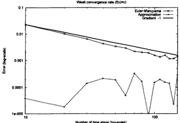
odd ffinction.

Through Figure 1 to Figure 3, x-axis denotes the number oftime steps $n$ until time 1

Rom 10 to

150

with logarithmic scale. Weak

errors

of simulation results

are

reported at

a

logarithmic scale

on

the

y-axis,

that

is

$|E[f(X_{1})]-E[f(\overline{X}_{1})]|$ (thin line) and _{$|E[f(X_{1})]-$}

$E[f(\overline{X_{\sim_{1}}^{\sim}})]|arrow$ (dotted line), where to obtain their

expectation

values,

we use

the Monte-Carlo

method with $10^{7}$ simulations for each _$n$

.

If they

are

parallel to the thick straight line, the

convergence

ratehas the order 1.

Thenumericalresultin the

case

of$f(x)=x$_{is the following:}

Weakoonvergencerate$(x)r)$

10 100

Number$othm\cdot t\cdot p\cdot(Q\infty 0)$

Figure 1: No. of time steps -weak

error

$(f(x)=x)$

.

From Figure 1, it is easytofind that the

convergence

rateofthe Euler-Mamyamamethod

has order 1, but for the Euler-Mamyama methodwith the approximated drift, the

approxi-mation converges

muchfaster than the uncorrected

one.

5.2 Case:

$\theta_{1}=-\theta_{0}=1$

and

$f(x)=\mathscr{K}$

Here

we

use

the

same

values of parametersintheprevious section andlet$f(x)=x^{2}$

.

From

Karatzas and Shreve [3,Exercise6.5.3,pp.441],

we

have

$E[X_{t}^{2}]=\frac{1}{2}+\sqrt{\frac{t}{2\pi}}(|x|-t-1)\exp(-\frac{(|x|-t)^{2}}{2t})+\{(|x|-t)^{2}+t-\frac{1}{2}\}\Phi(\frac{|x|-t}{\sqrt{t}})$

$+e^{2|x|}(|x|+t- \frac{1}{2})[1-\Phi(\frac{|x|+t}{\sqrt{t}})]$ ,

where set

(12)

Andin the

case

of$x=0$and$t=1$,

we

obtain$E[f(X_{1})]=0.333369$

.

Thenumerical resultinthe

case

of$f(x)=$ isthe following:

Weakconvergencerate$(f(x)-^{A}2)$

$tO$ tOO

Numberoftme steps(log-scale)

Figure2: No. oftimesteps-weak

error

$( \int(x)=x^{2})$

.

FromFigure2,

we

easily findthat the rate ofconvergence in the both methodsis 1.

5.3 Case:

$\theta_{1}=-\theta_{0}=1$

and

$f(x)=1(x>0)-1(x\leq 0)$

Inthis section,

we use

$f(x)=1(x>0)-1(x\leq 0)$which does not have regurality and does

notbelong to

our

theorem. Note that the fimciton$f$is symmetricwithrespect to the origin

a.e.

and$X_{t}$hasthecontinuousandsymmetric density fimction

so

that

we

have$E[f(X_{1})]=0$

.

The numericalresult inthe

case

of$f(x)=1(x>0)-1(x\leq 0)$ is the following:

Weakconvergence rate$(f(x)^{-}-ind|cator)$

70 100

Number of bmesteps$\{\log-\infty de)$

(13)

FromFigure3,it

is easy

tofindthat the

convergence

rateofthe Euler-Maruyama method

has order 1, but

as

before the Euler-Mamyama method with the approximated drift,

con-verges

faster.

We

have

testedthree

cases

above,the weak

convergence

rate

of

theEuler-Mamyama

ap-proximation in all ofthem is 1. And

in

the

case

oftheEuler-Mamyamaapproximation with

the approximateddrift,

we

couldnotobtain therate of

convergence

becausethe

approxima-tion

converges

too fast for$f(x)=x$and $1(x>0)-1(x\leq 0)$,butfor$f(x)=x^{2}$_,

we

find that

the

convergence

rate is 1. This is probably due to how $\epsilon$ is chosen. In this case,

we

have

chosen this examplebecause

we

can

obtain the weak limitin closed form. In orderto have

slowerorders,

we

need toconsider

more

complicated

situations.

References

[1] R.F.Bass,_Diffusionsand Elliptic Operators,Springer,1998.

[2] K.S. Chan and O. Stramer, Weak Consistency

_of

the EulerMethod

_for

Numerically SolvingStochastic

DifferentialEquations with Discontinuous Coefficients, Stoch. Proc. Appl. 76(1998),33A4.

[3] I. Karatzas and S.E.Shreve,BrownianMotionandStochasticCalculus,2nded.,Springer, 1998.

[4] P.E. Kloeden and E. Platen,Numerical Solution

_of

Stochastic_DifferentialEquations, 3rded., Springer,

1999.

[5] A.Kohatsu-Higa,A. Lejay,and K.Yasuda,Approximationmethods

_for

stochastic

_differential

equations

withnon-regular

_drift

(2012). Inpreparation.

[6] N. Krylov, An inequalilyinthetheory_ofstochasticintegrals, Th. Probab. Appl. 16(1971),438A48.

[7] O.A. Lady\v{z}enskaja, V.A.Solonnikov,and N.N.Ural’ceva,LinearandQuasilinear Equations

_ofParabolic

Type,AmericanMathematicalSociety, 1967.

[S] V.Mackevi\v{c}ius, On theconvergencerate

_of

Euler scheme

_for

SDE with Lipschitz

_drift

andconstant

dif-fusion, Proceedings oftheEigth Vilnius ConferenceonProbability Theoly and MathematicalStatistics,

Part I(2002),2003,pp.301-310, DOI 10.$1023/A$: 1025754020469.

[9] R. Mikulevi\v{c}iusand E.Platen,Rate_ofconvergence

_of

the Eulerapproximation_{for diffusion}processes,

Math. Nachr. 151(1991),233-239, DOI 10.$1002/mana$.19911510114.

[10] P. Przybylowicz, The Optimality

_of

Euler-type Algorithms

_for

Approximation

_of

Stochastic_Differential Equations with Discontinuous Coefficients,2010.Presentation slide.

[11] A. J. Veretennikov, Onstrongsolutions and explicit

_fomulasfor

solutions

_of

stochastic integral

equa-tions,Math.USSR Sb.39(1981),no.3, 387-403, DOI 10.$1070/SM19Slv039n03ABEH001522$

.

[12] B. L.Yan, The Euler Scheme with IrregularCoefficients,Annals ofProbability30(2002), no.3,