Inventory Control Policy for Repair Parts

Society of Japan

Vol. 38, No. 3, September 1995

INVENTORY CONTROL POUCY FOR REPAIR PARTS

Yasuo Kusaka Masao Mori

Tokyo Metropolitan college of Commerce Tokyo Institute of Technology

(Received April 1, 1992; Revised January 6, 1995)

A bstract The inventory control of repair parts has recently become an important subject in rationalizing logistics department. Information network systems for repair parts are being constructed. The purpose of this study is to propose a fixed interval ordering policy for repair parts of single item and clarify its effects. The proposed policy specifically takes into account the characteristic of repair part demands ocurring for corrective and preventive maintenance (CM and PM) and the predictability of PM demand. A new fixed interval ordering policy is discussed for negligible lead time in case where PM demands are predictable and thus their distributions are known from the first to the n-th period. In the analysis, it is theoretically clarified that the optimal expected inventory control cost decreases monotonously with respect to an increase in the predictable periods n for PM demand. It is shown that this policy can also be applied to a fixed interval ordering system considering lead time. Finally, some quantitative effects are examined by numerical examples. The proposed policy, based on the stratification of CM and PM demands and the wide-range prediction of PM demand, is considered to be effective in repair parts inventory control under information network.

L Introduction

The inventory control of repair parts has recently become an important subject in ra-tionalizing logistics department. Information network systems (INS) [4J for repair parts are being constructed. The reason for this is the necessity to respond quickly to user calls and reflect repair informations derived from corrective maintenance (CM) and preventive main-tenance (PM) in service and design for increasing sales of products. Such a network system enables us to improve the demand forecasting capability, transfer informations quickly to various fields and improve the adaptability to change. However, the hardware system of information network (IN) only offers the infrast.ructure for inventory control. To design a new control policy for giving intelligence to the system is a subject for effective operation of this system.

In conventional studies on inventory control, many models have been treated from various viewpoints: probabilistic models, dynamic demand models, perishable models, joint order models, models under the restriction of fund and production, speculative models and so forth [8J. (For example, we can show recent researches which discuss the joint ordering in multi-product inventory control [1], [3], [7] and research which discusses the reduction of set-up time and ordering lead time in production and inventory control system from the viewpoint of investment [2J.) In these models, the reductions of lead time and inventory through decreasing demand forecast errors and of ordering cost through taking into account the scale economy, have been important viewpoints for cutting down inventory control cost. However, in many conventional researches, almost no considerations have been given to the characteristics of both treated product demands and of IN.

270 Y. Kusaka & M. Mori

of single item and clarify its effects. The characteristics of repair parts demand and IN are reflected in this policy. That is, it is considered that (1) the repair parts demand can be stratified into CM and PM demands, and (2) wide-range PM demands can be predicted on real time base through INS. Specifically, the inventory control policy is formulated by stochastic dynamic programming (SDP) with respect to a case, where PM demands are predictable from the first to a certain period in a finite planning horizon and these probability distribution are known by a retrieval function of INS. Then, this policy is compared with the conventional policy supposing that PM demands are unpredictable for the planning horizon and the whole demand (the sum of CM and PM demands) follows a certain probability distribution. We treat, as ordering policy, a fixed interval ordering policy which enables us to utilize effectively PM demand informations for a finite planning horizon.

In Chapter 2, a fixed interval ordering policy is treated with respect to a case where lead time is negligible. In Section 2.1, a new policy is proposed for fixed interval ordering system in case where PM demands are predictable over the planning horizon and compare it with the conventional policy supposing that the PM demands are unpredictable over the planning horizon. In Section 2.2, as a generalization of Section 2.1, a fixed interval ordering policy is formulated in case where PM demands are predictable from the first to the n-th period. Then, the effect of optimal policy is examined theoretically in case where the predictable periods n of PM demand change. In Chapter 3, Chapter 2 is generalized by taking lead time into account. Sections 3.1 and 3.2 correspond to Sections 2.1 and 2.2, respectively. In Chapter 4, the effects of the proposed ordering policy are shown by some numerical examples using PM demand informations, and some important viewpoints are clarified for repair parts inventory control in INS. In Chapter 5, conclusions of this study are stated.

2. Fixed interval ordering policy with negligible lead time

2.1 The case of PM demands being predictable over the planning horizon 2.1.1 Fixed interval ordering policy using PM demand forecasting informations

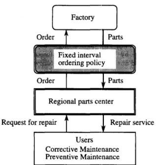
As indicated in Fig. 1, suppose a system for supplying a certain type of repair parts of products which need maintenance, such as copy machines, calculators and construction machines, at a regional parts center. The repair parts are dispatched on order from the factory to the regional parts center, stored as parts inventory and used for maintenance (CM and PM) to product users. In inventory control, two ordering policies are considered: fixed interval ordering policy and ordering point policy [6J. In this study the fixed interval ordering policy is treated because (1) the products should be made smoothly in factory, and (2) PM demand forecasting informations predetermined according to the periodicity of plan can be introduced into the policy effectively. Then, the maintenance activities to the users are important factors for increasing the sales of products. Therefore, we are concerned with effectively constructing a repair parts inventory control system at the regional parts center. Suppose that the maintenance department performs PM and CM for a large number of products used in market as shown in Fig. 2. Any PM or CM needs replacing one unit of repair parts. Generally any replacement affects a lifetime of operating parts in market. Since the replacement numbers of repair parts by PM and CM are sufficiently small compared with the number of operating parts in market, it can be considered the replacement by PM and CM has little influence on the whole lifetime distribution of operating parts in market.

PM is determined based on the maintenance capability and the use frequency for prod-ucts in market. This repair parts demand changes from the predetermined value due to the following reasons:

Factory

Regional parts center

Request for repair Repair service

Users

Corrective Maintenance Preventive Maintenance

Figure 1 Inventory control system of repair parts at regional parts cent er

,

•

Operating products

~

• PM candidates

r--t

PM

I

i

i

J

~I

CM

I

:

....

,--~

... _ .. __ .. __ ... , ... __ .. __ ... __ ... J

Figure 2 PM and CM activities for products in market

(1) Products for which PM has been planned are excluded from the PM list, because either some of products have failured and thus CM has been executed or others have practical use frequencies less than the pre-estimated value.

(2) Products for which PM has not been planned in advance suddenly come into PM, because these practical use frequencies have much ex.:eeded the predetermined value.

To be sure, PM and CM demands are dependent in the sense that PM demand tends to decrease if CM demand increases. However, we suppose that these changes in PM demand, especially the changes from PM to CM, are small compared with the mean value, and the CM demand is considered to randomly occur from operating parts in market from Drenick's Theorem.

In these circumstances, it can be considered that PM and CM demands are approximately and mutually independent and these empirical probability distributions are estimated from the retrieval function of data base in INS.

Specifically, an inventory control problem for repair parts using the fixed interval ordering policy is examined with respect to a case where PM demands are predictable over a finite

272 Y. Kusaka & M. Mori

planning horizon. Here, it is our subject how to construct effectively an inventory control policy for repair parts based on PM demand informations obtained from INS.

2.1.2 Formulation

In Section 2.1, we propose a fixed interval ordering policy which reduces the demand forecasting errors and inventories by using PM demand forecasting informations. Before proceeding to the formulation and analysis, we define the following term and notations: Term and notations

i-th ordering cycle (i = 1,·· ., T) : period from the i-th time point of order (or arrival) to the (i

+

l)-th time point of order (or arrival) for products, which is hereafter called the i-th period

Xci CM demand in the i-th period (discrete random variable) Xpi PM demand in the i-th period (discrete random variable) Xi

==

Xci

+

Xpi whole demand in the i-th period (discrete random variable)

<Pci(Xc;) probability distribution of CM demand in the i-th period <Ppi(Xpi) probability distribution of PM demand in the i-th period

<Pi(Xi) probability distribution of whole demand in the i-th period /-lci,O"ci : mean and standard deviation of Xci

/-lpi,O"pi : mean and standard deviation of Xpi /-li,O"i : mean and standard deviation of Xi

M : ordering cycle.

Ii inventory just before the order (or arrival) in the i-th period

Yi : ordering quantity in the i-th period

Zi

=

Ii

+

Yi inventory immediately after the arrival in the i-th period

hi : holding cost per unit of repair part in the i-th period ki : ordering cost in the i-th period (fixed cost)

Ci : ordering cost per unit of repair part in the i-th period (variable cost)

Pi : stockout penalty cost per unit of repair part in the i-th period

v : cost for disposing one unit of repair part inventory at the end of the planning horizon

X~i,T)

=

(Xpi, ... ,XpT ) : PM demand series from the i-th to the T-th period (discrete

random variable).

\lfi(x~i,T») : joint probability distribution of X~i,T)

8( .) = {I if Yi

>

0

y, - 0 if Yi

=

0

Assumptions

Under the circumstances described in 2.1.1, we assume the following conditions: (1) The random variables Xci and Xpi are mutually independent.

(2) The probability distributions <Pci(Xci), <Ppi(Xpi) and <Pi(Xi) are known. (3) The probability distributions for each period are mutually independent.

(4) The lead time for order is considered negligible. That is, it is assumed that repair parts arrive at the same time as ordering.

(5) PM demand series x~l,T) is predictable over the planning horizon. (6) All the demands in ordering cycle generate approximately uniformly.

Based on the above assumptions, the fixed interval ordering policy discussed in this study is illustrated in Fig. 3.

Inventory

·

:x. : I

·

·

·

·

~+1

=

1;+1

+

Yi+l

..

~

...

·

·

·

.~

...

:

.

. . I • I

·

·

·

·

·

~+2

=

Yi+2

·1·

~~,~~:---~.~--·---~.~.--~Time • I " • • I " I

·

'"

'.

: M •. I ... \.( ... ~ :....:: ••• _ •••• _ ••••••••••• ~ __ • __ J't ... __ •• .,:

· i -th ordering cycle: (i

+

1) -lh ordering cycle

Figure 3 Fixed interval ordering policy in case of negligible lead time Criterion

The ordering quantity (or inventory immediately after the repair parts arrival at the beginning of every period) is determined to minimize the expected inventory control cost for the planning horizon.

Conventional fixed interval ordering polic:y

When the inventory Ii just before the order at the beginning of the i-th period (i

=

1" ", T) is given, we minimize the expected inventory control cost incurred from the i-th period to the end of the planning horizon, based on the probability distribution of whole demand cI>j(Xj) (j = i, i

+

1" ", T), assuming that PM demands are unpredictable over the planning horizon. We call this policy as "conventional fixed interval ordering policy". Under this policy, the minimum value 9i(Ii) of expected inventory control cost from the i-th period on is given by the following equation (under the assumption (6), with respect to the average holding cost for both cases where the stockout occurs or does not occur, see the literature

[5], p. 91):

Z,

+

L {(

Zi - xd2)hi

+

9i+1 (Zi - Xi)}cI>i( Xi) :1:,=0

00 z~ ]

+

L

{(Xi - Zi)Pi

+

2~' hi

+

9i+l(O)}cI>i(Xi)

~=~+1 I

for Vi

=

1,2"", T; VIi 2: 0

for VIT+l 2: 0 (2.1)

Here, kih(Zi - Ii)

+

Ci(Zi - Ii) within brackets [

1

at the right hand side of 9i(Ii) represents the

Zi

ordering cost for ordering quantity (Zi - Ii). The part within braces of

L { }

at the right :1:,=0

274 Y. Kusalw & M Mori

hand side relates with the inventory control cost in case where inventory exists at the end of the th period; the first term of the above-mentioned part is the average holding cost in the i-th period under i-the assumption (6), and i-the second term is i-the minimum expected inventory control cost in case of starting with the inventory Zi - Xi at the end of the i-th period and

00

following the optimal policy during the remaining periods. The part within braces of

L: { }

zi+1

relates with the inventory control cost in case where stockout occurs in the i-th period; the first term of the part is the stockout penalty cost, the second term is the average holding cost under the assumption (6) and the third term is the minimum expected inventory control cost in case of starting with inventory 0 at the end of the i-th period and following the optimal policy during the remaining periods. The equation 9T+1(IT+1) = vIr+1 represents the cost for disposing the inventory parts at the end of the planning horizon.

Proposed fixed interval ordering policy

Consider the ordering policy which minimizes the expected inventory control cost in-curred from the i-th period to the end of planning horizon based on the conditional prob-ability distribution iPj(Xj/xVT»)(j

=

i, i

+

1" ", T), supposing that the inventory

Ii

just before the order at the beginning of the i-th period (i = 1"", T) and PM demand series

x~i,T)

for the remaining planning periods are predictable. Under the proposed fixed interval ordering policy, the conditional minimum expected inventory control cost fi(Ii/x~i,T») for the remaining periods from the i-th period on, given that x~i,T) is as follows:

+

fi+1

(0/x~i+1,T»)

_}iPi(

Xi/x~i,T»)]

for Vi = 1,2, ... , T; VIi

2::

0 h+1(IT+t!xf+1,T») = vIr+1 for _VIT+1

2::

0,

(2.2)

h h I" ( / (iT») I" ( / (i+1,T») I" ( / (i,T»)

were t e relations Ji+1 Zi - Xi xp' Ji+1 Zi - Xi xp and Ji+1 0 Xp =

fi+l(O/x~i+l,T») are used, noticing that the optimal policy from the (i

+

l)-th period

on is determined based on PM demand series x~i+1,T). At the beginning of the (T

+

1)-th period, 1)-the inventory is only disposed and 1)-the x~T+1,T) has no substantial meaning. Moreover, it is necessary to note that the following relation holds:

iPi(xi/x~i,T») = iPi(xi/xpi)

=

{~Ci(Xi

- Xpi)

for Xi

<

Xpi otherwise

The optimal inventory in every period, where PM demand series x~l,T) is unpredictable over the planning horizon, can be obtained by solving the equation (2.1). Also, the optimal inventory at the beginning of every period in case of x~l,T) being predictable can be obtained by solving the equation (2.2).

As x~l,T) is a realized value of all the possible PM demand series, it is necessary to evaluate the effect of the proposed policy based on the following equation. The equation

takes into account all the occurrence possibilities of x~l,T) in order to clarify the effect of the proposed method compared with the conventional one. Using the joint probability distribution ll1i(x~i,T») of x~i,T), this criterion is expressed by

!;(Ii):=

L

ll1i(x~i,T»)fi(Idx~i,T») for Vi = 1,2, ... , T; VIi ~ 0

x~i,T) _(2.3)

2.1.3 Analysis

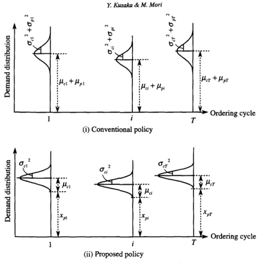
From (2.1) and (2.2), we can find that the essential difference between the conventional and proposed fixed interval ordering policies lies in the following point: in the former the optimal policy is determined based on the proba,bility distribution <I>j(xi) since probability distribution of PM demand series X~l,T) is unpredictable, while in the latter it is deter-mined based on the conditional probability distribution <I>i(xdx~i,T») since the distribution of X~l,T) becomes known. In order to clarify the difference, the relation between <I>j(Xi)

and <I>i(xdx~i,T») is shown in Fig. 4. Denoting the expectation and variance of random variable W by" E(W) and V(W), respectively, we have the relations E(Xi) = Ilci

+

/lopi and

E(Xi/x~i,T»)

=

/loci+Xpi from the relation Xi = Xcj+Xpi in Fig. 3. We have also the relation

V(Xi) = a;i

+

a\

>

a;i = V(Xdx~i,T») from the assumption (1). Since the safety stock of the proposed poficy is considered to be less than that of the conventional policy from the relation V(Xi)

>

V(Xdx~i,T»), it is expected that the proposed policy is more economical than the conventional one, that is, the relation fi(Ii)

S

9i(Ii) holds. Hereafter, we will prove theoretically the above relation in case where the joint probability distribution of X~l,T) is known.

Lemma 1. With respect to a function Ui(Zi; Xi) composed of decision variable Zi and non-negative random variable Xi, the following relation holds (the proof is omitted):

Lemma 2.

E

ll1i(x~i,T»){ ~n

f:

Ui(Zj;

Xi)<I>i(xdx~i,T»)}

x~,T) Xi=O

00

S

ll}!n

E

Ui(Zi; X;) <I> I (Xi)

Xi=O

The equation (2.3) is rewritten

fi(Ii) =

x~O

<I>pi(Xpi)

~ri

[kib(Zi - I;)

+

Ci(Zi - Ij)

Zi

+

E

{(Zi - xi/2)hi

+

fi+l(Zi - Xi)}<I>i(xdxp;) Xi==O

00 ~ ]

+

L

{(Xi - Zi)Pi

+

;~hi

+ fi+l(O)}<I>i(x;jX pi)

xi=zi+l .• X,

for Vi ==: 1,··· ,TjVIi ~ 0 for VIr+! ~ O.

276

~

+

-r·-

_, ,

.

_, ,

l.uc1

+

.upl , ,

y. Kusaka & M. Mori

t

b

+

·r·-L----.L...II---iL..-l---'T~~ Ordering cycle

(i) Conventional policy

·1-·-, .u

el

_·x-··

_, , , , ,

:x

p1 , , , ,

·1-··

_

.~.~eT

, _, , , ~ xpT , ~---~~---~I---~~Orderingcycle T 1

(ii) Proposed policy

Figure 4 Structure of demand distributions in conventional and proposed fixed interval ordering policies

(The proof is given by Appendix 1.)

Lemma is used actually for calculating fi(Ii).

Using Lemmas 1 and 2, it is proved that the following property holds with respect to the relation between the minimum expected inventory control cost h(Ii) in the proposed policy and the cost 9i(Ii) in the conventional one:

Property 1.

fi(Ii) ~ 9i(Ii)

(The proof is given by Appendix 2.)

for 'Vi = 1,2, ... T : 'VIi ~ 0

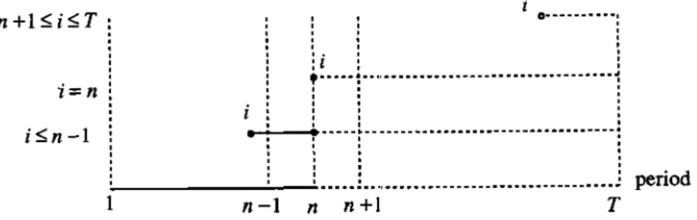
2.2 The case of PM demands being predictable from the first to the n-th period 2.2.1 Formulation

Property 1 indicates the importance of forecasting PM demand in designing the inven· tory control policy for repair parts. The degree of forecasting capability of this PM demand

depends on the performance of PM planning system itself and INS incorporated. It is con-sidered that the more the forecasting capability is improved, the less the inventory control cost is. Accordingly, in this section, we formulate, as a generalization of the problem ex-amined in Section 2.1, a fixed interval ordering policy in case where PM demands from the first to the n-th period are predictable and thus these probability distributions are known. We theoretically clarify that the inventory control cost is reduced by improving forecasting capability in the sense of the predictable periods n being longer.

Before proceeding to formulation, we define newly introduced notation rf(Ij). Other terms and notations are almost same as those in the preceding section.

rf(Ij) : Suppose that PM demand series is predictable from the first to the n-th period and is unpredictable for the remaining periods from the (n

+

1 )-th period on. Then, given the inventory Ij just before the order (or arrival) in the i-th period, the minimum expected inventory control cost from the i-th period on under the optimal policy is defined as rf(Ij). n+l~i~T 0---·--····: , i=n , ' , _,. ' _' :l . : t-· .. --~.-" -_ .. -_ ... _ ... -_ ... -_ ... _ ... _ ... ~ , , ' , ' , ' , ' , ' , , , i~n-l

...

~-

.... , ... -r ... -_ ... -.. --._._ ... ---:

, ' , ,

:...-_ _ _ _ _

.:..--...:. _____ ! __ .. ________________________________

~ period n-1 n n+l T

Figure 5 Relation between decision period j: and PM demand fore casing periods n

period in which Xpi is predictable. - - - period in which Xpi is unpredictable.

As indicated in Fig. 5, PM demand is unpredictable for any period i with n

+

1 ~ i ~ T. In case of i

=

n, PM demand is predictable in the i-th period while it is unpredictable from the (i

+

l)-th period on. In case of i ~ n - 1, PM demand is predictable between the i-th and n-th periods while it is unpredictable from the (n

+

1 )-th period on. Also, in cases of n = 0 and n = T, PM demands correspond to the cases where PM demands are respectively unpredictable and predictable over the planning horizon, as treated in Section 2.1. From the above, the following recurrence equation holds with respect to ri(Ii):

for n =1= 0, T; Vi = n

+

1,"" Tj VIi ~ 0 for n =1= O,T;i

=

njVIi ~ 0

for n =1= O,l,TjVi = 1" ",n -ljVIi ~ 0 for n

=

OjVi

=

1"" ,TjVIi ~ 0

for n

=

TjVi

=

1"" ,TjVIj ~ 0 r!}+l(IT+l)=vIT+l for n =O, .. ·,TjVIr+l ~O,

where 9i(Ii) and fi(Ii) are given by the equations (2.1) and (2.3) respectively, and Qil(Ii)

==

f:

<Ppi(Xpi) min

[ki~(Zi

- Ii)

+

Ci(Zj - Ij)

x --0 z;'?.!.

278 y. Kusaka & M. Mori

z,

+

L

{(Zi - xi/2)hi

+

9i+l(Zi - Xi)}<Pi(xi/xpi)

x,=O

z,

+

L

{(Zi - xi/2)hi

+

rf+1(zi - Xi)}<Pi(xi/Xpi)

x,=O

00

Also,

L

<Ppi(Xpi),in caseofn#O,Tji=n and n#0,1,TjVi=1,···,n-1,isaddedin

Xp,=O

order to take into account all the possibilities of x~i,n), by the similar reasoning of converting

h(Ii/x1

i,T») in (2.2) into !i(Ii) in (2.3).

2.2.2 Analysis

Generally, it is considered that the optimal inventory control cost is reduced as the predictable periods n of PM demand increase. This is shown theoretically as follows: Property 2.

for Vn = 0"", T - 1j VIi ~

°

(The proof is given by Appendix 3.)

Property 2 indicates that the more improved PM demand forecasting capability, the less the inventory control cost is. The reduction value in the optimal expected inventory control cost rf(Ii) under the proposed policy, compared with the cost r?(Ii) = 9i(Ii) under the conventional one, is given by

Cn(Ii)

=

9i(Ii) - rf(Ii).

From Property 2, it is seen that Cn(Ii) is non-decreasing with respect to n. The reduction value Cn(Ii) is an index for judging how much effect is brought about by improving the PM demand forecasting capability. That is, it represents the "information cost" which is bearable for obtaining the demand forecasting capability n.

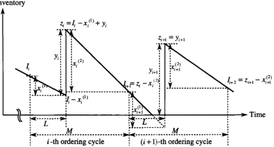
3. Fixed interval ordering policy taking lead time into account

3.1 The case of PM demands being predictable over the planning horizon In Chapter 2, we discussed the fixed interval ordering policy in case where PM demands are predictable over the planning horizon and thus these probability distributions are known. In Chapter 3, we discuss the fixed interval ordering policy considering lead time (L

<

M), excluding the assumption (4) of Chapter 2. The fixed interval ordering policy in this case is illustrated in Fig. 6. In the figure, the whole demand of repair parts from the order to the arrival in the i-th period (the sum of CM demand and PM demand) and the whole

Inventory _ / (I) Z;- i-Xi +Yi

•••

, Yi+l: , ' : (2~

,

·+r

Z; -Xi :

.T...

:

:1-X.<I) , I 1 , , , , , , , , ~~~---~~---~~~~"~+---~--~Time }oII( ••••••••• ~ :4:···t···~ .. ~ : L : ~f

__

.!:' __ ..

_:~m.; : ' M _{:...: •••••••.•.••••.••.••••••••.••••••• .:.0.: ... . :} ' M ' 1 i -th ordering cycle 1 (i

+

l)-th ordering cycle 1

Figure 6 Fixed interval ordering policy considering lead time

demand from the arrival up to the order in the (i

+

1 )-th period are defined as x~1) and

x~2), respectively. The CM and PM demands, which compose x~1) and x~2), are denoted by

x~~), x~!), x~;)

and

x~~),

respectively. Moreover, their probability distributions are denoted by (1)( (1)) (1) (1)) (2) (2) (2) (2) . . . ' .

cl> ci xci ,cl>'p_{i (Xpi} ,cl> ci (Xci ) and cl>'p_{i (Xpi ),} respectIvely. Let I" YI and Ii be the Inventory just before the order in the i-th period, the ordering quantity and the inventory immediately after the parts arrival, respectively. Then

I:

is expressed by

for x(l)

_,

<

_- l-

_,

for

xP)

~

Ii

+

1.

Given the inventory Ii just before the order at the beginning of the i-th period, the minimum expected inventory control cost on and after the i-th period under the conventional fixed interval ordering policy, 9i(1i), is given by the following equation from Fig. 5, in the same way as (2.1):

280 Y. Kusaka & M. Mori

for Vi = 1"" ,TjV1i ~ 0

for VIT+l ~ 0, (3.1 )

where r

==

iT,

hil

==

rhj and hi2

==

(1 - r)hi. On the other hand, the minimum expected inventory control cost fi(Idx~i,T») on and after the i-th period, under the proposed fixed interval ordering policy, is given by the following equation in the same way as (2.2):

. [ Ii x(l)

h(Idx~"T»)

=

mi~

kiO(Yi)

+

CiYi

+

E

[(Ii -

T

)hil

~? x0)=o

.

Zi (2)

+

E

{(Zi - x~ )hi2

+

fi+l(Zi - x~2) /x~i+l,T»)} X 4i~2)(x~2) /x~i,T») X\2)=O

00 2

+

E

((x~2)

- Zi)Pi

+

Z~2)hi2

+

fi+l(O/x~i+l,T»)}

x(2)=Zi+l 2Xi

X 4i~2)(x~2) /x(i,T»)] 4iF)(x~l) /x~i,T»)

~

[(1) . .

tt .

+

L..J (Xi - I,)p,

+

---wh'l

X\1)=Ii+1 2xi

Yi (2)

+

E

{(Yi - X~ )hil

+

fi+l(Yi - x~2) /x~i+l,T»)}4i~2)(x~2) /x~i,T»)

X\2)=O

00 2

+

E

{(x~2)

- Yi)Pi

+

Y~2)hi2

+

fi+l(O/x~i+l,T»)}

x\2)=y.+l 2Xi

for Vi = 1," . , Tj V Ii ~ 0

(3.2)

As x~i,T) is a realized value of all the possible PM demand series, it is necessary to evalu-ate (3.2) based on all the occurrence possibilities of x~i,T), in order to clarify the effect of the proposed system through comparison with the conventional method. Using the joint probability distribution \If i(x~i,T») of x~i,T), this criterion is expressed by

h(Ii)

==

E

\Ifi(x~i,T»)fi(Idx~i,T») for Vi = 1,,,, ,TjVlj ~ 0

X~·,T) (3.3)

Ii [X~l) Zi X(2)

+

E

(1i - T)h i1

+

E

{(Zi - T)h i2 X\l)=O X\2)=O

+

!;+l(Zi - X~2»)}<I>~2)(X~2) /X~~»)

00 2

+

E

((X~2)

- Zi)Pi

+

Z~2)

hi2

+

!;+!(0)}<I>~2)(X~2) /X~;»)l

( 2) 2x·

Xi =zi+l I

for Vi = 1,· .. , Tj VIi 2 0

(3.4)

for VIr+! 2

o.

It is proved that the following property holds with respect to the relation between !;(1i) and 9i(1i), by using the similar method as Property 1 (the proof is omitted).

Property 3.

for Vl: = 1, ... , Tj VIi 2 0

3.2 The case of PM demands being predictable from the first to the n-th period In this section we formulate, as a generalization of the problem discussed in the preceding section, a fixed interval ordering policy in case w here PM demands are predictable from the first to the n-th period and thus these probabi:lity distributions are known. Then, in the same ~ay as discussed in Section 2.2, we can show that the inventory control cost reduction is brought about by improving forecasting capability in the sense that predictable periods n

become longer.

The notation rf(1i) is used in the same meaning as Section 2.2. Using equations (3.1) through (3.4), the following DP recurrence equation holds with respect to rf(1i):

where

for n

#

O,TjVi = n

+

1, ... ,TjVIi 20 for n..J. O.T·i ., j '

=

n·VI· ,1_

>

0

for n = 2, ... , T - 1; VIi 2 0 for n = 0; Vi = 1, ... , Tj VIi 2 0 for n = Tj Vi = 1, ... , Tj VIi 2 0 for n = 0,···, T;VIr+l 20,

282 y. Kusaka & M. Mori

~(2)( (2)/ (2))] ~(1)( (1)/ (1))]

x ~I XI X_pI ~I XI X_pI

It is shown that the following property holds in the same way as Property 2, with respect to predictable periods n of PM demand and rf(Ij) (the proof is omitted):

Property 4.

4. Numerical examples

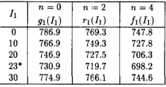
In Properties 2 and 4 it has been clarified theoretically that the cost of proposed policy decreases gradually as the predictable periods n of PM demand increase. However, the degree of cost reduction has not been made clear. Therefore, in this chapter the effects of the proposed policy are clarified by sensitivity analysis for some numerical examples. Table 1 shows the parameters, where PM demand Xpi consists of the sum of a constant d p

and a Poisson variable with rate Ap , and CM demand Xci follows a Poisson variable with rate Ac , for every period i in inventory control with negligible lead time and a planning

horizon of 4 periods. Table 2 shows the expected inventory control cost under the optimal policy (hereafter called "optimal expected inventory control cost") based on the parameters indicated in Table 1, for five types of initial inventory

It

in the first period and for three cases of PM demand in the planning horizon being unpredictable (n = 0), partially predictable (n = 2) and completely predictable (n = 4). The

Ii

means the initial inventory

It

that minimizes 91(It),

rr(It)

and !I(1!). This table indicates that the effect of cost reduction increases as the predictable periods n of PM demand increase.

Table 1 Values of parameters

dp

=

15; Ap

=

2; Ac

=

3; T == 4; n

=

0,2,4

ki

=

10, Ci

=

2; hi

=

10; Pi == 100 (i

=

1 '" 4); v

=

5

Table 2 Changes of

It,

n and optimal expected inventory control cost with negligible lead time

It

n=O n:= 2 n=4 91(1!)

rdh)

h(h)

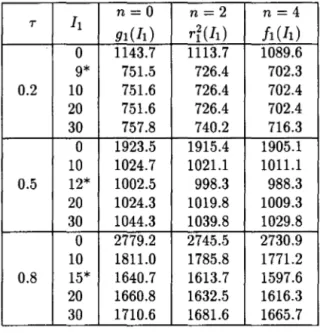
0 786.9 769.3 747.8 10 766.9 749.3 727.8 20 746.9 72:7.5 706.3 23* 730.9 719.7 698.2 30 774.9 766.1 744.6

Table 3 shows the optimal expected inventory control cost with lead time for three values of T

=

0.2, 0.5, 0.8 (the proportion of lead time in one period), the five types of

initial inventory

h

and the same three cases of PM demands as Table 2. The parameters are same as Table 1. The effect of cost reduction becomes large as the predictable periods n increase. This table also indicates that less initial inventories are economical as the lead time decreases while they are extremely expensive as the lead time increases. Therefore, it becomes more important to control the increase ;m inventory cost by holding an appropriate initial inventory as the lead time increases or to reduce the lead time itself by constructing IN.

From the above, longer predictable periods n of PM demand and shorter lead time should be adopted as much as possible for more effective inventory control. It is considered that the proposed policy, based on the stratification of C M and PM demands and the consideration of PM demand predictability, is effective in INS.

2B4 Y. Kusaka & M. Mori

Table 3 Changes of h, n and optimal expected inventory control cost with lead time

h

n=O n=2 n=4 T gl(h) ri(h) h(h) 0 1143.7 1113.7 1089.6 9* 751.5 726.4 702.3 0.2 10 751.6 726.4 702.4 20 751.6 726.4 702.4 30 757.8 740.2 716.3 0 1923.5 1915.4 1905.1 10 1024.7 1021.1 1011.1 0.5 12* 1002.5 998.3 988.3 20 1024.3 1019.8 1009.3 30 1044.3 1039.8 1029.8 0 2779.2 2745.5 2730.9 10 1811.0 1785.8 1771.2 0.8 15* 1640.7 1613.7 1597.6 20 1660.8 1632.5 1616.3 30 1710.6 1681.6 1665.7 5. Conclusion

In this study a fixed interval ordering policy was proposed for repair parts of single item over a finite planning horizon, considering the characteristic of repair part demands occurring for CM and PM and the predictability of PM demand. Using SDP, a fixed interval ordering policy was formulated in case where the lead time was negligible, and it was theoretically shown that the optimal expected inventory control cost decreased as the predictable periods of PM demand became longer. Then, it was shown that the analysis was also applicable to a fixed interval ordering policy considering lead time. Finally, some quantitative effects of the proposed policy were given by numerical examples. The proposed policy is considered to be effective in repair parts inventory control under INS.

References

[1] Aggarwal, V.: "A Closed-Form Approach for Multi-item Inventory Grouping", Naval Research Logistics Quarterly, Vol. 30, pp. 471-485, 1983.

[2] Beek, P. and Putten, C.: "OR Contributions to Flexibility Improvement in Produc-tion/Inventory Systems", European Journal of Operational Research, Vol. 31, No. 1,

pp. 52-60, 1987.

[3] Charkravarty, A. K.: "Multi-Item Inventory Aggregation into Groups", Journal of Op-erational Research Society, Vol. 32, No. 1, pp. 19-26, 1981.

[4] Hanaoka, S.: "Business Strategy and Information Network in Changing Era" (in Japanese), Nikkan Kogyo Shimbunsha, 1989.

[5] Kitahara, T. and Kodama, M.: "Inventory Control System by OR", (in Japanese), Kyushu University Press, 1982.

[6] Mizuno, Y.: "Introduction to Inventory Control" (in Japanese), Nikka-giren, 1974.

Com-mon Cycle" (in Japanese), Journal of Japan Industrial Management Association, Vol. 38, No. 2, pp. 120-125, 1987.

[8] Tinarelli, G. U.: "Inventory Control: Models and Problems", European Journal of Op-erational Research, Vol. 14, pp. 1-12, 1983.

Appendices

Appendix 1: The Proof of Lemma 2 Proof.

Noticing that there holds ~i(xi/x~i,T») == ~i(xi/xpi) in (2.2) and Wi(x~i,T))

=

~pi(Xpi)Wi+1(X~i+1,T») from assumption (3), the following relation holds from (2.2) and

(2.3):

1i(I;)

=

L

Wi(x~i,T) fi(Ii/x~i,T»)

X~;,T) 00 ='

L

~pi(Xpi)

L

Wi+1(X~i+1,T»)Ji(Ii/x~i,T») Xp;=O X~;+l,T) 00 =

L

~pi(Xpi)

L

Wi+1(x1i+1,T»)x Xp;=o X~;+l,T)

~~

[kib(Zi - I;)

+

Ci(Zi - Ii)

~ X' .

+

L

{(Zi - 2')hi

+

fi+1(Zi - xi/x~'+1,T)}~i(xi/xpi)

x;=O

00 ~ ]

+

X;~+l

{(Xi - Zi)Pi

+

2~i

hi

+

fi+1(O/x1i+1,T»)}~i(Xi/Xpi)

=

f:

~pi(Xpi)

min [kib(Zi - Ii)

+

Ci(Zi - Ii)+

x _{p . -}·-0 z,,?,I;

+

t

{(Zi -

~i)

+

L

Wi+1(x1i+1,T))fi+1(Zi -

xi/x~i+1,T»)}

x

~i(Xi/xpi)

x;=O X~+l,T)

00 2

+

L

{(Xi - Zi)Pi

+

!.Lhi

+

L

Wi+1(X~i+1,T»)fi+1(0/x1i+1,T»)}

X;=Z;+l 2x, X(O+l,T)

p

(A2.1)

Applying 1i+1(Zi - Xi) =

L

Wi+1(x1i+1,T»)fi+1(Zi - xi/x1i+1,T») and fi+1(0) =

(;+l,T)

Xp

L

Wi+1(x~i+1,T»)fi+1(0/x1i+1,T») to the last equation at the right hand side of

X~+l,T)

(A2.1), the result follows. 0

286 y. Kusaka & M. Mori

Proof. The proof is given by mathematical induction. When i

=

T

+

1, from (2.1) and Lemma 2, we have

for 'VIT+l ~

o.

(A2.2)

Therefore, h+l(IT+l) ~ 9T+l (IT+l) holds. Next, we show that h(Ii) ~ 9i(Ii) holds generally, supposing

for 'Vi = 1,·· ., T; 'VIi+l ~ 0 (A2.3) holds. Applying Lemma 1 to Lemma 2, and using the induction assumption of (A2.3) and (2.1), we have

h(Ii)

~ ~~~ x~O

<Ppi(Xpi) [kpib'(Zi - Ii)

+

Ci(Zi - Ii)

Zi Xi

+

L

{(Zi - "2)hi

+

fi+l(Zi - Xi)}<pi(xi/xpd Xi=O

00 Z~ ]

+ XiE+l {(Xi - Zi)Pi

+

2~/i

+

h+l(O)}<Pi(xi/Xpi)

=

~~

[kib'(Zi - Ii)

+

Ci(Zi - Ii)

Zi xi

+

L

{(Zi - "2)hi

+

fi+l(Zi - Xi)}<Pi(xi) Xi=O

00 ~ ]

+

Xi~+l

{(Xi - Zi)Pi

+

2~i

hi

+

h+1(O)}<Pi(Xi)

~

min [kib'(Zi - /j)

+

Cj(Zi - Id zi?Ii

Zi Xi

+

L

{(zi-"2)hi +9i+1(Zi- Xi)}<Pi(Xi)

Xi=O

00 z7 ]

+

Xi~+l

{(Xi - Zi)Pi

+

2~i

hi

+

9i+1(O)}<Pi(Xi)

= 9i(Ii).

Thus, the proof is complete.

o

Appendix 3: The Proof of Property 2 Proof.

(i) the case of 1 ~ n ~ T - 1

<D

n

+

2 ~ i ~ T (n ~ T - 2)

From (2.4), we have ri+1(Ii)

=

9i(Ii) and ri(Ii)

=

9i(Ii). From this, the relation rf+l(Ii) ~ ri(Ii) holds.

®i=n+1

From (2.4), we have

rf+1(1i) =

f:

cI>pi(xpd min [ki15(Zi - Ii)

+

Ci(Zi - Ii)

X p.---0 zi?Ii

Zi

+

L

{(Zi - x;/2)hi + 9i+1(Zi - Xi)}cI>i(X;/Xpi) (A3.2)

Xi=O

DC

Applying Lemma 1 and the relation cI>i(Xi) =

I:

cI>pi(Xpi)cI>i(X;/Xpi) to the right hand side

Xpi==O

of (A3.2) and using (2.1), we have

rf+1(1i) :::;

~~~

[kic5(Zi - Ii)

+

Ci(Z'i - Ii)

+

x~O

{(Zi - x;/2)hi

+

9i+1(Zi - Xi)}cI>i(Xi)

00 z7 ]

+

L {(

Xi - Zi)Pi

+

2~ _ hi

+

gi+1 (O)}cI>i( Xi)

Xi=Zi+1 I

= 9i(1i).

From (A3.1) and (A3.3), the relation rf+1(1i) :::; rf(1i) is obtained.

@i=n

From (2.4), we have

ri(Ii) =

f:

cI>pi(Xpi) min [kic5(Zi - Ii)

+

Ci(Zi - Ii)

X p.---0 zi?Ii Zi

+

L

{(Zi - x;/2)hi

+

9i+1(Zi - Xi)}cI>i(x;jxpi)

Xi=O

+

f:

{(Xi - Zi)Pi

+

2Z;~hi

+

9i+1(0)}cI>i(x;j XPi)]

Xi=Zi+ 1 • I

ri+1(h)

=

f:

cI>pi(Xpi) min [kic5(Zi - Ii)

+

Ci(Zi - Ii)

X p . ---0 zi?Ii Zi

+

L

{(Zi - x;/2)hi

+

r~tl(Zi - Xi)}cI>i(X;/Xpi)

Xi=O

As i = n, the following relation hold from the result of

® :

ritl(zi - Xi) :::; ri+1(Zi - Xi) = 9i+1(Zi - Xi) ritl(O) :::; ri+1(0) = 9i+1(0).

(A3.3)

(A3.4)

(A3.5)

(A3.6)

Applying the relations (A3.6) to r~l(zi - Xi) and rithO) at the right hand side of (A3.5) and using (A3.4), the relation ri+ 1(1i) :::; rf(Ij) is obtained.

2BB Y. Kusaka & M. Mori @1:::;i:::;n-1

When i = n - 1, the relation ritl(1i+I) :::; rf+1(1i+t) holds from the result of @. Generally, we will show the relation ry+1(1i) :::; rf(1i) for Vi = 1,···, n -1; VIi

2:

0 assuming that there holds ritl (1i+1) :::; rf+1 (1i+1) for Vi = 1, ... , n - 1; V1i+1

2:

O.

From (2.4), ri(1d is the equation obtained by substituting n

+

1 into n in (A3.5). The equation ri+1(1i) is given by the equation (A3.5) itself. Applying the induction assumption to the terms ri":l(zi-Xi) and ritl(O) at the right hand side of (A3.5), and using the equation

ri(1i) obtained from (A3.5), the relation ri+1(1i) :::; ri(1d is obtained. (ii) the case of n = 0

(D2:::;i:::;T

From (2.4), we have the relations ri+1(1i)

=

9i(1i) and rf(1i)

=

9i(1i).

From this, the relation ri+1(1i) :::; ri(1i) holds.

@i=1

From (2.4), we have

ri(1i)

=

9i(1i)

ri+1(li)

=

f:

CPpi(Xpi) min [kit5(Zi - 1i)

+

Ci(Zi - 1i)

x _{p . -}'-0 Zj?Ij

Zi

+

L:

{(Zi - xd2)hi

+

9i+1(Zi - Xi)}CPi(Xi/Xpi)

Xi=O

00

(A3.7)

(A3.8)

Applying Lemma 1 and the relation CPi(Xi)

=

L:

CPpi(Xpi)CPi(Xi/Xpi) to the right hand side of equation (A3.8) and using (2.1), we have

r~+l(L)

_{I I}

<

_{- Zj?Ij} min [k.t5(z' -_{I I} L) _I

+

c'(z' -_{I I} L) _I

Zi

+

L:

{(Zi - xd2)hi

+

9i+1(Zi - Xi)}CPi(Xi) (A3.9)

Xj=O

+

f:

{(Xi - Zi)Pi

+

2Z

!'

hi

+

9i+1(O)}CPi(xd]

Xj=zi+1 I

=

9i(Ii)

From (A3.7) and (A3.9), the relation ri+1(1i) :::; rf(I;) is obtained. From (i) and (ii), the

proof has been completed. 0

Yasuo Kusaka

Department of Business Management Tokyo Metropolitan College of Commerce 1-2-1 Harumi, Chuo-ku, 104, Japan