On the Stability of Vehicular Traffic Flow-A Phenomenological view point

Vol. 8, No. 3, June 1966.

ON THE STABILITY OF VEHICULAR TRAFFIC

FLOW-A PHENOMENOLOGICAL VIEWPOINT

DA VID H, EV ANS

Research Laboratories General ,Motors Corporation Warren, Michigan

(Received Jun. 8, 1965) ABSTRACT

An attempt is made to explain the cause of instability in vehicular traffic flow by assuming that the equilibrium flow of a system is related to the concentration of vehicles in the system by a parabolic curve. Measurements of tunnel and freeway traffic are the basis for this as-sumption. I t is found that the flow for densities less than that for maximum flow, i.e., the unsaturated flow regime, is completely stable. On the other hand the saturated flow regime is unstable to certain perturbations but will support finite oscillations. Finite oscillations between the two regimes can be either stable or unstable, but in particular oscillations around maximum flow are unstable.

INTRODUCTION

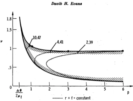
The general bchavior of traffic flow as a function of concentration IS well known, at least qualitatively, for many systems. Examples of such systems are single lane flow in tunnels for which there is good quantitative data [ 1] and multi-lane flow on freeways where the situation is more difficult [2]. This behavior of the steady state flow is shown schematically in Fig. 1 where the abscissa is the number of vehicles in the syssem at one time and the ordinate is the flow in vehicles per unit time. The solid line represents the gross or averaged flow and the circles represent data points. The average flow increases linearly at first with

On the Stability of Vehicular Traffic Flow 135 the number of vehicles in the system but as the number of vehicles increases the flow reaches a maximum and then drops off and finally breaks up. The scatter in the data points, of course, is because the flow and the number of vehicles are both statistical quantities and subject to fluctuations. Large fluctuations indicate the onset of ins-tability and it is this effect that we want to investigate here.

We will use an extremely simple model. Fig. 2, which is an idealization of Fig. 1, shows the flow as a function of the number of vehicles in the system assuming that there are no fluctuations; we do not supply the reasons for such behavior but take this result as our starting point. For simplicity we take the flow curve to be a parabola following Helly [3] who worked with the discrete case. We assume that this curve determines the dynamic behavior of the system and thus have restricted our considerations to the slowly varying case. We further assume the flow out of the system is equal to this flow. Finally, we assume that the flow into the system is independent of the number of vehicles in the system-at least up to the point where the flow out is zer0 when the model breaks down.

If we let N Ct) be the number of vehicles in the system at time t it then follows that

where

_d:: =q(t)-rN (2M-N),

O~N(t)<2M,

q(t)=flow into system, vehicles per unit time, r=constant,

( 1 )

Jl;[=constant, the number for which the system has maximum flom out.

tn writing down Cl) we have assumed that the flow out is immediately affected by any change in the input flow. As is well known a similar

physically unrealizable condition obtains for the heat equation. Such a change in the flow out is patently unrealizable for a well defined bottleneck downstream of the input. However, if the bottleneck is ill defined or distributed as for example can be the case in multilane flow on a more or less homogeneous highway, it seems reasonable that there should be a regime where (1) is a valid approximation to a physical system. Remarks akin to these can be made about the validity of the assumption that the flow in is an independent variable. Unfortunately because of the present state of the theory of vehicular traffic flow no quantitative limits can be put on the regime of validity; the plausibility of the model must rest on the results which can be obtained from it. Two results which will be obtained which argue in favor of plausibility are (l) the instability of the flow to a small change in the input on the retrograde side of the flow curve, which would thus cause the scatter in measured data, and (2) the impossibility of maintaining a flow at maximum, which is not documented but is noised about.

2. PRELIMINARY ANALYSIS

For mathematical convenience we set (see the dashed axes III

Fig. 2) so that becomes r;=(N-M)/M w=q/rM2 7:=r M2t ( 2) (3)

The normalized flow out is [l-r;2] and thus for steady state flow a necessary condition is O::;;w::;; 1. The time variable 7: has a unit such

that if the system starts at time 7:

=

0 with no vehicles in it, r;

=

-1,

On the Stability of Vehicular Traffic Flow 137

vehicles are allowed to leave, then at time r= I we find that r;=0, i.e.,

the number of vehicles in the system is such that the flow is a maximum. The steady state solutions of (3) are obtained by setting w(r)=O, a constant, and dr;/dr=O. Then

r;(r)=±VCT':":o), for 0::;:0::;:1. ( 4)

The negative sign is for the unsaturated flow case and the positive sign for the saturated flow. Of course, these solutions were purposely built into the model.

Since we are interested in time varying solutions of (3) let us examine this equation from the mathematical viewpoint briefly. It is a Riccatti equation and is discussed in many places, e.g., Ince [4], Forsythe [5], Watson [6]. The substitution ~I=-V'/V linearizes it,

v" +[w(r)-I]v=O. (5 )

Ideally, analytic solutions to (3) or (5) for noiselike w(r) are desired. What is available, however, is the following: For w a constant the solution of (5) is trivial. For w a periodic function (5) is Hill's equa-tion and for the special case w=a+ ,3 C03 pr it is Mathieu's equation,

[ 4, 5] Whittaker and Watson [7], Stoker [8], McLachlin [9]. The periodic cases are difficult enough; apparently nothing has been done for more noiselike w. Thm there is little use for the existing literature.

3. CONSTANT INPUT

Let us set w(r)=O, a constant; we can then find r; straightforwardly by solving (5). It is convenient to define

p=+vll-OI,O::;:O. (6)

Case I: 0::;:0<1.

r;(r)=-p+2p [I+ P -+-_p 7i"-e

2I'c]-I,

r;(O)=r;o, r:::::O. (7) r;,.

1,'0<0, 1;(r) increases or decreases, as the case may be, smoothly to 1,'(=) = - p., a point in the unsaturated steady state flow region in Fig. 2. For O<1,'o<p. the same is true, i.e., starting at the point 1)0' 1) decreases

to 1) (=)

= -

p. while the flow increases to a maximum and then decreases toward its steady state value. On the other hand, for 1)o>f! the flow

decreases and 1) builds up to 1)= 1 so that the flow stops and the model breaks down. Hence, points representing flows which are to left of the maximum in Fig. 2 are stable to step function changes in the input while points on the retrograde sIde of the curve are unstable to step function changes because either the flow goes to the unsaturated con-dition or the flow breaks down no matter how small the change. As has already been remarked in the Introduction this behavior gives us an important plamibility argument for the validity of the model. Its importance is seen when the measurement of the statistics involved is considered. The measurement must take place during a finite length of time; if a step function change in input occurs during this time the instability would cause considerable scatter in the numerical results. Case II:

0>

1.

Clearly this case is transient

( 8 ) which is valid for O:S:; r< ro where 1) (ro) = 1.

There remains the transition case 0= 1 ; one finds that

(9) Thc solution is stable for 1)0:S:;0 and otherwise holds only for O:s:;r<ro where 1)(ro)=1.

4. SMALL OSCILLATIONS

Let us next consider the more noiselike case of an oscillatory input; put

On the Stability of Vehicular Traffic Flow 139

w(r)=a+f3cospr, a>O, 1f3I:S:a. (10) Since a is the average flow in the on'cy case of interest IS a:S: I and so we set

(11)

The differential equation (3) then becomes

(12)

A; already noticed the known asymptotic results for the Mathieu equa-tion, which i<; the equation (12) goe3 into when linearized by the sub-stit'ution r;=

-v' Iv,

do not appear to be useful to us. We therefore restrict the examination to the case 1(31 small and obtain a few terms of a perturbation expansion of r; in power.> of (3. We set

sub ;titute it into (12) and set the eocfficients of

f3

to zero; thus YO'_Yo2= _k2,

Yl' - 2YOYl

=

cos pr , Y2'-2YoYZ=Yl 2,

(13)

(14)

The analysis can be simplified by choosing the initial conditions judiciously. Let us set Yo(O)=k; the solution to the first of equation (14) i<; then

Yo(r:)=k, -I<k<+l. (15)

With the above sub3titution the second of equation (14) has the general solutlOa

For k negative the last term goes to zero as r: increases regardless of the initial canditions; for k~O the initial conditions can be chosen such that al =0 to pre~erve the oscillatory charader of the solution. We can

pro-ceed in a like manner for higher power3 of " and the results, except for k=O, are the same; that is, for k less than zero the solution is unconditionally asymptotically oscillatory, for k greater than zero the initial conditions may be chosen so that the solution is oscillatory. For the case k=O the solution (16), with al =0, reduces to

Yl(')=~

sin

pr.

p (17)

Substituting this into the third of equations (14) and solving we find

(18)

which is unstable for any choice of a2'

Summing up the results of this section we have found that (1) the flow is unconditionally stable to small oscillations in the input flow for flows represented by points to the left of the maximum in Fig. 2; (2) for input flows equal to the maximum flow in Fig. 2 the flow l~ unconditionally unstable to small oscillations, as had been mentioned in the Introduction; and (3) for flows represented by points on the retro-grade side of Fig. 2 the flow is conditionally stable to small oscillations.

5. FINITE OSCILLATIONS

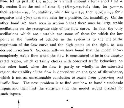
It is possible to investigate the stability under finite oscillatiom in the input by using the remIts for step function input" section 3. Suppose the input flow is the rectangular wave shon in Fig. 3. For a time T the input is Or and for a time

f

it is Of; without loss of generality we demand Or>O/. Then for stable oscillations during the time T, 1J will rise to a peak value 1J and during the following time

J,

r; will fall to its minimum value '2 and so on. Clearly

(19)

On the Stability of Vehicular Traffic Flow 141

7J. and ij must exist and, conversely, if they exi~t there is stability. The average value of the input flow is

and clearly must be restricted as indicated. I t is convenient to define

As before there are two cases: Cases I: O~Of<O,<l.

By the use of (7) it is found that

-pi+Ptfj

Pt-r;

where we have set

Pf=Pf cothfpf> pr=/l, coth rPr for convenience.

Ca,e II: O::::;Of<l<Or

From (7) and (8) it is found that

-pi+Ptfj

Pt-fj

where for this case we have set

Pf= Pf cothiJ, pr= pr cot rpr. (20) (21) (22) (23) (24) (25) (26)

(27)

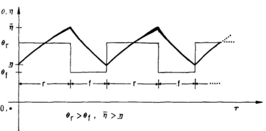
I t is instructive to plot these equations for some typical O's before analyzing the equations. Fig. 4 shows these equations superimposed on

one another. On the abscissa the values are plotted for PI and each of

the

pr's

and the

p's

are used as the indepenent variables; the values of

1 and 1; are plotted on the ordinate. A typical stable oscillation for Case I with 01=1/2 and Or=0.96<1 has ij=-1/4, 1=-1/2 with Pr

indicated by T and pr bye. A companion stable oscillation has 1;

=

1/2, 1

=

1/4 with the same value3 for Pr and pr which are now indicated by • and l::J., respectively. It is seen generally from thi~ figure that only two kinds of stable oscillations exist for this case: - Pr<"'L<1;< - pr

<0

or O<pr<r;<1;<Vr. For Case

n,

0r=1/2, Or=1.04<1, a typical stable o,cillation has 1;=-1/4,7,'=-1/2 with Pr still the value indicated by ... but pr now indicated by 0; the companion oscillatIOn 1;=1/2, 72= 1/4 again exists. A type of stable 03cillation not allowed under the previous case has 1;=1/4, 1=-1/2 with

Pt

indicated by

0

and pr«O)

indicated by

x,

the companion o,cillation has 1; = 1/2, l',1= -1/4. General-ly it is clear from the figure that a necessary condition for stable oscillations is - PI

<r; <f;

<PI.

Let us now obtain the general conditions for stability; we will only analyze the more interesting case, Case

n,

for which Or>1. By combining (25) and (26) we obtain the following quadratic equation for 7j:

(28)

The quadratic equation ij satisfies is the same except that the sign of the middle term is negative. It is expedient to introduce the definitions

p=pr+PI, LlO={}r- Or=pr2_+pr2_{, (29)} whcrc the last is from (21). Thc solutions of (28) are then

1£= -(LlO/2p)2±

v7{

(30)

where

(31)

On the Stabillty 01 Vehicular 1'raffic INow

respective denominators and then eliminating the terms

ii·

TJ... between

these equations that for any solution 1)

fJ

=r;+t1(} /

p .

(32)

By (29) and (19) necessarily

p>o.

(33)

From Fig. 4, as already mentioned, or by analysis, It is necessary that

(34)

Thus the necessary condition for stable oscillations is

(35)

where the left limit must obviously be non-positive and the right limit non-negative.

First let us look at the requirement that R be non-negative. We

can define lJ such that

(36)

where the last is from (33) and (27). A convenient mixed notation for

R as a function of lJ is (37) For R to be positive (38) where (39) For

p

large,

i.e.,

rand

f

small, it can be shown that (39) implies (20). Next from the signs of the limits in (35) it is seen that

(40) which further restricts the range of

p.

Also, (40) can be found directly

by the instructive method of letting

J

be infinite, which means that

Pj=Pj,

setting7J=-Pf, ~=+pj, and then solving for

p.

Finally, under the assumption that the previous conditions, (38) and (40), are satisfied, the remaining inequalities in (35) give only

(41) which adds nothing that was not already known; however, it is reas-suring. The canstants (39), (40), (41) all have the point

p=iJ(J/2pj

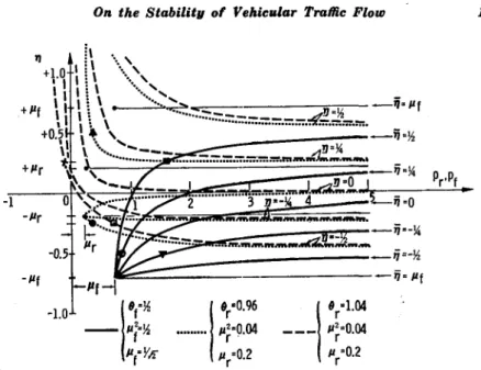
in common on their boundaries.

In Fig. 5 the area defined by the above constraints has been ~ketched for the case considered before, namely OJ= 1/2, Or= 1.04. The parameter p is some sort of a generalized frequency because of the behavior of its components

pr

and

PI.

To show the precise relation between rand

J

and the stability criterion three of the curves

r+ J=

constant have also been plotted in Fig. 5. Clearly the qualitative aspects of the stability criterion will not change with the value3 of Or and

(J

j .

The results for Case I, fJr

<

1, are not particularly interesting.

Briefly, oscillations of the variety >;'<o<~ are not allowed; on the other hand for any 7{, ij such that - pj<7J<~<

-

pr or pr<r;<~<pj there exist compatible chocies of

pr

and

PI.

6. CONCLUSIONS

The model we have used in investigating the stability of vehicular traffic flow, which is all contained in equation (I) in its physical form, appears to have a range of validity. The evidence for this statement is all qualitative and it is not clear at this time how to obtain quanti-tative validation. Some of the qualiquanti-tative evidence has already been given in the Introduction, i.e., the derivation of the equation and some results. The same effect found using the step function can be illustrated in another way: Suppose these is a steady state flow with 7j=7jo which

On the Stability of Vehicular Tralnc Flow 145 Now let us perturb the input by a small amount e for a short time

a.

By tection 3 at the end of time iJ, 7/(tl)=r;o=1)o+eo; thus, for 1)o=-p.o then 1)(oo)=-p.o,

i.e.,

stability, while for 7jo=+P.J then 1)(oo)=-p.o for 0:

negative and 1) (00) does not exist for e positive, i.e., instability. On the

other hand we have seen in section 5 that there may be large, stable oscillations on the retrograde side of the flow curve. In fact the only oscillations which are unstable are some of those for which the low point in the number of vehicles in the system is to the left of the maximum of the flow curve and the high point to the right, as was derived in section 5. So, essentially we have found that the model shows completely stable flow when the flow is constrained to be in the unsatu-rated region, which certainly checks with observed traffic behavior; on the other hand, when the flow is partly or wholly in the saturated region the stability of the flow is dependent on the type of disturbance, which is not an unreasonable conclusion to reach from observing real traffic flow. The next problem is to find out how to handle stochastic inputs and then find the statistics that the model would predict for such inputs.

Flow

•

•

,

_,

•

,

\ \ \

.

\ \ L -________________________________________________ . _

Number of Vehicles

Fig. 1. Schematic representation of the flow vs. the number of vehicles in a system showing scatter of data points about average.

q max Flow

N=O

11 =-1

t

M

I

o

Unsaturated

_I

Saturated

2M

+1

Fig. 2. Idealization showing flow as a parabolic function of number, N, of vehicles in system. Normalized flow vs. normalized number, 1), is shown by dashed axes, see equations (2).

0, 'i'J ----M+t---.f

-+-...

0,· .... ... T

Fig. 3. Schematic drawing of rectangular wave input into system, wC:"). and resultant steady state variation of number in system,

r/,).

Here, max r;(,)

-1

"

+1.0 -Pr -0.5 -lit -1.0

On the Stability of Vehicular TraRic Flow

\ , \

.•.

',

...

_...

"

-=:--'---..::;-;----ij= "l IftIftHft . . ".." . . . . , . ... ~_---::::;r]r.:.-=lr--ij.-J4 ••• Irr .... """'''' ... ~ ... IW\, . . .

r/~~=======·-ii=-~

~ -'i=P!

pr-l

'(~ 112=\2 f P(Y~

'r

cO .96

";=0.04

Pr =0.2 147

Fig. 4. Surerimposed curves with the values for the variables 7) and fj given on the ordinate and the values for pr and PIon the abscissa. Three families are shown: the dependent variable '11 as a function of the independent variable PI for the parameter (h= 1/2 and for various initial values ij, the variable ij as a function of pr for 8=0.96 and various initial!l> and the variable ij as a func-tion of pr for 8r

=

1.04 and various initial '11.

1.8 1.5 v _2.39 ~ .5 0 1 1 1 1 I-

I

..

AS 1 2 3 4 5 6 2Pf _{r + f = constant} P

Fig. 5. The region bounded by hatched lines gives IJ, p for which stable

oscillations exist for the case (Jf=1/2, 8r =1.04. Constant period curves are indicated by the dashed lines with periods (in units of r) as shown. On such curves r decreases monotonely from its value on the upper curves, IJ=.A(p), and goes to zero as the curve asymptotically approaches the lower curve, IJP=Pf.

ACKNOWLEDGMENTS

The author wishes to acknowledge the understanding gained by many conversa-tions with his colleagues, Robert Anderson, Robert Herman, and Richard Rothery, at the General Motors Research Laboratories.

REFERENCES

[1] R. Herman and R. Rothery, "Microscopic and Macroscopic Aspects of Single Lane Traffic Flow", Opns. Res. (Japan) 5, 74 (1962).

[2] A.F. Malo, H.S. Mika and V.P. Walbridge, "Traffic Behavior on an Urban Expressway", Highway Research Board Bull. 235, NRC Publication 698 (1960). [3] W. Helly, "Two Stochastic Traffic Systems Whose Service Times Increase

with Occupancy", Opns. Res., 12, 951-963 (1964).

[4] E.L. Ince, Ordinary Differential Equations, Dover, New York, 1944.

[5] A.R. Forsyth, A T"atise on Dijforcntial Equations, 6th edition, Macmillan, London, 1943.

On the Stability of Vehicular Traflic Flou 149 (6) G.N. Watson, A Tre2ti:e o.~ the Theory of Eessel Functions, 2nd edition,

Cambridge, 1952.

(7) E.T. Whittaker and G.N. Watson, A Course of Modern Analysis, American edition, Macmillan, New York, 1947.

(8) J.J. Stoker, Nonlinear Vibrations, Interseience, New York, 1950.