HPhi_exercise.key

HΦの演習問題 (解説)

好きなものからやって下さい

ほとんど

_{laptop PCでできるはずです(TPQはちょっと重いですが…)}

もちろん、自分のやりたい別の課題もやっても

_OKです

三澤 貴宏

東京大学物性研究所 特任研究員（PCoMS PI）

例題1: spin 1/2 dimer (full diag)

例題2: spin 1/2 chain (Lanczos)

例題3: J1-J2 Heisenberg model(Lanczos,TPQ)

例題4: Kitaev model (Lanczos,TPQ)

Basic exercise !

いくつかのサンプルは以下のサイトにあります

https://github.com/yomichi/HPhi-samples

例題

1:

反強磁性

S = 1/2 Heisenberg dimer

最も簡単な量子系のひとつである 反強磁性

2

_{S = 1/2}

Heisenberg dimer model

H = ⃗S

1

· ⃗S

2

ただひとつの基底状態とみっつの縮退した励起状態とがある

基底状態は全スピン Stot = 0 で、エネルギーは E = −3/4 励起状態は全スピン Stot = 1 で、エネルギーは E = 1/4

最初の一歩としてこれを

HPhi

で解く

2_{以下特筆なければすべて反強磁性模型です}

©Y.Motoyama

例題

1: S = 1/2 Heisenberg dimer

入力ファイル

SpinHalf.def

1

model = " SpinGC "

2

lattice = " chain ␣ lattice "

3

method = " F u l l D i a g "

4

2 S = 1

5

L = 2

6

J = 0.5

これを

HPhi

の

Standard

モードで処理するだけ

SpinGC

の

GC

は

Grand Canonical

J = 0.5

なのは周期的境界条件のためボンドが

2

本あるから

1

> HPhi -s S p i n H a l f . def

3 / 17

余裕があれば

, S=1, S=3/2…などをやってみましょう(2S=2などとするだけ)

Emin=-S(S+1), Emax=S^2になるはずです

_©Y.Motoyama

例題

2: S = 1/2 Heisenberg chain

入力ファイル

StdFace.def

1

model = " Spin "

2

lattice = " chain ␣ lattice "

3

method = " Lanczos "

4

2 S = 1

5

2 Sz = 0

6

J = 1.0

7

L = 12

Spin

は

Canonical

2Sz

は 計算したい状態の全スピンの

z

成分の

2

倍

今回は低エネルギー状態のみでいいので

Lanczos

法を使う

1

> HPhi -s StdFace . def

例題

2-A: S = 1/2 Heisenberg chain

S = 1/2 Heisenberg chain

H =

!

Li=1

S

⃗

i

· ⃗S

i+1

周期境界

S

L+1

= S

1

を課す（以下同様）

基底状態は朝永・

Luttinger

流体で、ギャップレス

励起は線形分散を示す

有限系では状態の取れる波数が離散化されるため、エネルギー

ギャップが開く

分散が線形なので、∆ _{∝ 1/L} となる 3

有限系のエネルギーギャップを

HPhi

で計算する

3_{実際には対数補正がかかる} 5 / 17

©Y.Motoyama

例題

2: S = 1/2 Heisenberg chain

入力ファイル

StdFace.def

1

model = " Spin "

2

lattice = " chain ␣ lattice "

3

method = " Lanczos "

4

2 S = 1

5

2 Sz = 0

6

J = 1.0

7

L = 12

Spin

は

Canonical

2Sz

は 計算したい状態の全スピンの

z

成分の

2

倍

今回は低エネルギー状態のみでいいので

Lanczos

法を使う

1

> HPhi -s StdFace . def

例題

2: S = 1/2 Heisenberg chain

今回も大量の出力とともに一瞬で計算が終わる（はず）

必要な情報は

output/zvo_Lanczos_Step.dat

に出力されて

いる

4

1

> tail -n 3 output / z v o _ L a n c z o s _ S t e p . dat

2

stp =42 -5.3873909174 -5.0315434037

-4.7773893336 -4.5693744101

3

stp =44 -5.3873909174 -5.0315434037

-4.7773893337 -4.5693744108

4

stp =46 -5.3873909174 -5.0315434037

-4.7773893337 -4.5693744108

これは各

“Lanczos step”

で計算した「ちいさい固有値」が幾

つか並んでいる

デフォルト設定では第一励起エネルギーの収束をチェックして

いる

これの左

2

つの差がエネルギーギャップ

4_{一応ログ出力にもほぼ同じのが出ている} 7 / 17

©Y.Motoyama

例題

2: S = 1/2 Heisenberg chain

データ抽出の自動化

一回だけなら電卓に手入力でもいいけれど、超絶面倒くさいの

で自動化すべき

tail

と

awk

でワンライナーを書くのが楽

5

1

> tail -n 1 output / z v o _ L a n c z o s _ S t e p . dat

| awk ’{ print ␣ $3 - $2 } ’

2

0.3 558 48

長さ

L

を変えながらエネルギーギャップ

∆

を何度も計算して、

ギャップの長さ依存性を見てみよう

ノート

PC

、特に仮想マシンでは

L = 18, 20

ぐらいで止めてお

くのが賢明

それ以上のサイズは自習時間にがんばってください

L

を変えて何度も計算するという操作も自動化を試みてみよう

→ 次のページ 5_{自分の手に馴染んでいるなら何使ってもいいです} 8 / 17

©Y.Motoyama

例題

2: S = 1/2 Heisenberg chain

入力の自動化 今回はひとつのパラメータを変えるだけなのでシェルで事足 りる 共通となるパラメータをくくりだして保存しておく (StdFace.common) 1 model = " Spin "

2 lattice = " chain ␣ lattice "

3 method = " Lanczos " 4 2 S = 1 5 2 Sz = 0 6 J = 1.0 別々のL 毎にこの共通ファイルをコピーして、足りないパラ メータを追記すればよい 1 rm -f res . dat 2 for L in 10 12 14 16; do

3 cp StdFace . common StdFace . def

4 echo " L = $L " >> StdFace . def

5 HPhi -s StdFace . def

6 gap = $ (( tail - n1 \

7 output / z v o _ L a n c z o s _ S t e p . dat |\

8 awk ’{ print ␣ $3 - $2 } ’)

9 echo $L $gap >> res . dat

10 done

ヒアドキュメントを使うのもアリ。自分の好きなようにやりま しょう

9 / 17

©Y.Motoyama

例題

2: S = 1/2 Heisenberg chain

結果

S = 1/2 Heisenberg chain

はギャップの閉じるぎりぎり

のところにあり、

log L

の対

数補正が現れるので結構数値

解析が難しい

0 0.1 0.2 0.3 0.4 0.5 0 0.02 0.04 0.06 0.08 0.1 \Delta 1/L a + b*x Lanczos

S = 1/2 XY chain (J

z

= 0, J

x

= 1.0)

ではもっと綺麗にかける

→

練習問題

・

S=1 Heisenberg chainにするとギャップが見えるはず(Haldane gap)

→練習問題 [input fileで 2S=2 とするだけ]

©Y.Motoyama

例題3: J1-J2ハイゼンベルク模型

lattice.gpで描画可能

H = J

₁

X

hi,ji

S

_i

S

_j

+ J

₂

X

hhi,jii

S

_i

S

_j 0 3 00 1 12 0 4 0 15 0 5 0 7 0 13 1 0 11 2 13 1 5 1 12 1 6 1 4 1 14 2 1 22 3 14 2 6 2 13 2 7 2 5 2 15 3 2 33 0 15 3 7 3 14 3 4 3 6 3 12 4 7 44 5 0 4 8 4 3 4 9 4 11 4 1 5 4 55 6 1 5 9 5 0 5 10 5 8 5 2 6 5 66 7 2 6 10 6 1 6 11 6 9 6 3 7 6 77 4 3 7 11 7 2 7 8 7 10 7 0 8 11 88 9 4 8 12 8 7 8 13 8 15 8 5 9 8 99 10 5 9 13 9 4 9 14 9 12 9 6 10 9 1010 11 6 10 14 10 5 10 15 10 13 10 7 11 10 1111 8 7 11 15 11 6 11 12 11 14 11 4 12 15 1212 13 8 12 0 12 11 12 1 12 3 12 9 13 12 1313 14 9 13 1 13 8 13 2 13 0 13 10 14 13 1414 15 10 14 2 14 9 14 3 14 1 14 11 15 14 1515 12 11 15 3 15 10 15 0 15 2 15 8

最近接 J1,次近接J2

J2/J1 0.5で非磁性の

基底状態(スピン液体?)

HONG-CHEN JIANG, HONG YAO, AND LEON BALENTS PHYSICAL REVIEW B 86, 024424 (2012)

Most of the literature on the intermediate phase of the J1-J2

model has focused on the possibility of symmetry breaking VBS order. Many of these prior studied have suggested that the intermediate state has VBS order. We note, however, that all numerical results for the J1-J2 model are based

either on biased techniques (such as series expansion or coupled cluster methods, or fixed node or related versions of Monte Carlo adapted to avoid the sign problem, which is present for unbiased Monte Carlo in this system), or on exact diagonalization of very small systems. Some theoretical motivation for the possibility of VBS order comes from the theory of deconfined quantum criticality,28 _{which predicts}

that a continuous quantum phase transition—a deconfined quantum critical point (DQCP)—should occur between an ordered Ne´el state and a plaquette or columnar VBS state, in some models. However, the existence of such a transition does not in any way imply that it occurs for the J1-J2 model in

question, or that this particular model even harbors a VBS phase. Other theoretical motivation for VBS order comes from its presence in some large-N generalizations of the nearest-neighbor Heisenberg antiferromagnet. However, these large N studies are not controllably close to the SU(2) case and, moreover, do not consider second-neighbor interactions. In short, we believe there is very little compelling evidence for the existence of VBS order in the isotropic S = 1/2 J1-J2

model to be found in the prior literature. We will return to discuss VBS states in Sec. VI A.

The only unbiased technique capable of treating generic frustrated two-dimensional spin systems of moderately large size is the density matrix renormalization group (DMRG) method.7,29–31 _{While the sizes that can be studied using the}

DMRG are not as large as those accessibly by quantum Monte Carlo (QMC) for unfrustrated models, they are still very large and they are not limited by the sign problem, which prevents application of QMC to most realistic physical models. Moreover, the DMRG has some advantages over QMC: it is intrinsically a zero-temperature technique, and obtains a convenient representation of the ground-state wave function. Most importantly for our purposes, the DMRG is very efficient and convenient for calculating the entanglement entropy, which we return to in some detail below. In this paper, we report the results of extensive simulations (with truncation error ∼10−7_{) on numerous cylinders of}

circumfer-ence Ly = 3–14 and lengths Lx ! 2Ly. In our simulations, we

measure spin-spin correlation functions, correlation functions and expectation values of VBS order parameters, bulk singlet and triplet energy gaps, and entanglement entropy. All results confirm the existence of magnetic order for small and large J2,

and that (see Fig. 1) the ground state for 0.41 " J2/J1 " 0.62

is nonmagnetic, in very good agreement with the most accurate prior results from series expansion and coupled cluster24 methods. Furthermore, we find that the intermediate phase has a gap to both singlet and triplet excitations and, within our uncertainty, no VBS order in the 2D limit as extrapolated from the VBS correlation functions. We carry out further checks for possible finite-size effects due to the boundaries, to see if this might artificially suppress VBS order, and see no indication that this is the case.

The latter results suggests a QSL state, based on negative evidence: the apparent absence of VBS order. We find two

0.0 0.2 0.4 0.6 0.8 1.0 0.0 0.1 0.2 0.3 0.0 0.1 0.2 0.3 m_s(k₀) m_s(k_x) m s J₂/J₁ ∆ T _, ∆ S ∆_T ∆_S

Neel AFM Stripe AFM

QSL

FIG. 1. (Color online) The ground-state phase diagram for the spin-1

2 AFM Heisenberg J1-J2 model on the square lattice, as

determined by accurate DMRG calculations on long cylinders with Ly up to 14. Changing the coupling parameter J2/J1, three different

phases are found: N´eel antiferromagnet (AFM), topological quantum spin liquid (QSL), and stripe AFM phase. ms(k0 = (π,π)) [ms(kx =

(π,0))] denotes the staggered magnetization in the N´eel AFM phase [stripe AFM phase], whose saturation value is 1/2. "S and "T denote

the spin singlet and spin triplet gaps, respectively.

positive evidences that this suggestion is correct, and that the state is a Z2 QSL. First, we find a nonzero TEE, γ , which

is a constant and universal reduction of the von Neumann entanglement entropy, known to vanish in any gapped state with short-range entanglement. Notably, we point out in Sec. IV that discrete spontaneous symmetry breaking phases such as valence bond solids have absolute ground states, which are Schr¨odinger cat states with a constant enhancement of the entanglement entropy, i.e., an effect of opposite sign to the TEE. Phases with nonzero γ and a gap to all excitations are topological phases. Like conformal field theories in two dimensions, only discrete types of topological phases exist, with discrete allowed values of γ (which plays a role somewhat similar to the central charge in a conformal field theory). For all points we have studied within the nonmagnetic phase, the value of γ is equal, within numerical uncertainty of 2%, to ln(2), which is the minimal value possible for γ in a topological phase with time-reversal symmetry. A topological entanglement entropy of γ = ln(2) implies either a Z2 QSL

or a “doubled semion” phase. As there is, to our knowledge, no theory suggesting the appearance of the semion phase in an SU(2) invariant spin-1/2 model, we take this as strong evidence for a Z2 QSL state. The second positive evidence for

a Z2 QSL is a remarkable odd/even effect in which static VBS

order is entirely absent for even Ly but is observed directly

in the VBS expectation values for odd Ly. This is expected

on general theoretical grounds for a Z2 QSL, as we show

in Appendix 1. We compare the behavior of the numerically observed static VBS order for odd circumference cylinders with theory, and find quite consistent results.

The remainder of the paper is organized as follows. In Sec. II, we report results of magnetic and dimer correlation functions and their extrapolation to the infinite system limit. Section III discusses the singlet and triplet energy gaps. Section IV describes the theory and measurements of the topological entanglement entropy, and Sec. Vpresents results on the even-odd effect. We conclude in Sec.VIwith a summary of the conclusions, and a detailed discussion of the reasons to

024424-2

例題3: J1-J2ハイゼンベルク模型

H = J

₁

X

hi,ji

S

_i

S

_j

+ J

₂

X

hhi,jii

S

_i

S

_j

1. Lanczosでエネルギーを計算 (サイズ4 4位)

2. TPQで比熱を計算(J2/J1 0.5でどうなるか？)

3. (発展)余裕があればスピン相関も計算してみましょう

L =4

W = 4

model = "Spin"

method = "Lanczos"

lattice = "square lattice"

J = 2.0

J’ = 1.0

2Sz = 0

例題3: 基底状態の答え

4746

E.

DAGOTTO AND A.

MOREO

momentum

very

close

to

the

ground

state.

They

may

easi-ly

become degenerate

or

cross

in

the

thermodynamic

limit.

To

study this

excited (singlet zero

momentum)

state

with

our numerical

method

we

need

to

use

as

a

starting

configuration

a state

orthogonal

to

the

ground

state.

In

principle,

that

can be

accomplished

_by

selecting

as

a trial

function

the

state

~ y&,; ~&

=

~p& (p~ leap& ~ I/fp&,

where

~ p& is

arbitrary

(as

long

as

its

projection

on

the

excited

state

is

nonzero)

and ~ yo&

is

the

ground

state

previously

calculat-ed.

However,

we

found

that

in

practice

it is simpler

to

ob-tain

an

orthogonal

state

_{by inspection}

of

the

ground

state.

For

example,

if

two

states

~ ai&, ( a2&

of

the

S,

basis

ap-pear

in

the

ground

state

with

weights

_ai,

a2, respectively,

then

a state

orthogonal

to

the

ground

state

is

~ y&„,

,

~&

=

₍

_a

~&

—

a

~/az ~

a

2&.

This

is

the method

we used

and,

in

general,

it produces good results.

For

example,

evaluating

the

ground-state

energy

Eo

with

error

10

we

get

an

ac-curacy

of

10

in

the

energy

of

the

first

excited

state.

If

we

continue

the iterations

after

an

error

of

10

is

reached, the

state

decays

into

the

ground

state

because

originally

it

had

a

projection

on

the

ground

state

due

to

small

errors

in _a~,

az.

We

can generalize these

ideas

for

higher

excited

states,

but

of

course the

accuracy

of

each

—1.

0

new

excited

state

is

poorer than

the

previous

one.

Applying

this

technique

we found

the

remarkable

result

shown in

Fig.

4(a)

(some

special

values

of

the

energies

are

also presented

in

Table

I).

In

the

region

Jz=

(1.

1,

1.

5)

there

is

another

singlet

state

with

zero

momentum

(E~),

very

close

to

the

ground

state.

Note that

the gap

between

these

two

states

is

much

smaller than

the

_{gap between}

the

triplet

(ET)

and

the

singlet

(Eo)

states at

J2

=0

(see

also

Fig.

2)

which we know will

become degenerate

in

the

ther-modynamic

limit.

In

Fig.

4(a)

we

also

show

some points

corresponding

to

a

second

excited

state

(E2).

Those

values

have

error

bars

because

of

the

difFiculty in

stabiliz-ing

the

state

against a

decay

into

the

ground

state.

'

One

possibility

is

that

the

two

almost

degenerate states

are

the

equivalent

of

the

Neel

states

_{yo and} y&

of

Fig.

1

with

a

small

_gap

opened between them (which

is

possible

since

they

have

the

same quantum

numbers).

However,

if

an

interchange

of

states

effectively has

occurred

then

the

excited

state

should have

magnetic

properties opposite

to

those

of

the

ground

state,

as

_{yo and} y~ have on

the

8-site

lattice.

We

have

evaluated

the

magnetizations

in

the

ex-cited

state

and

they

are

qualitatively

very

similar

to

those

of

the

ground

state,

not

the opposite.

Then

we have

a

more interesting

situation

where

on

a

finite region

of

parameter

space the

lowest-lying levels

above

the

ground

state are

singlets

rather

than

triplets.

Consider,

for example, the

following

scenario:

Suppose

that

the

states

whose

energies

are

denoted

_by

Eo

and

_E2

(or

some

other excited

state)

in

_Fig.

4(a)

correspond

to

the

states

_{yo and y~} on

the

8-site lattice

(Fig. 1)

with

a

gap opened.

Then the

singlet

(E~)

of

Fig.

4(a)

is in

correspondence

_{with y2}

of

Fig.

1 which was

degenerate

with

the

ground

state at

one-point

on

the

8-site lattice.

'

Then

in

the

interval

J2=

(1.

_1,

1.

5)

we may have

a

new

disordered

ground

state'

'

(the

staggered

magnetiza-tions

are

very small in

that region). The

"one

point"

new

phase

of

the

8-site lattice

corresponds

now

to

a

finite

re-gion.

It

is very

dificult to

imagine

that

the

fact

that

the

lowest-lying

excited

states

are

singlets

rather

than

triplets

can be a

finite-size efI'ect.

Then,

we

conjecture

a

phase

di-agram

for

this model

as

shown in

_Fig.

4(b).

Since

the

magnetizations

behave

very

smoothly

we

expect

second-1.

3

0.

8

1.0

'1.

4

0.

0

I/////////I

V / / / / / / / / I

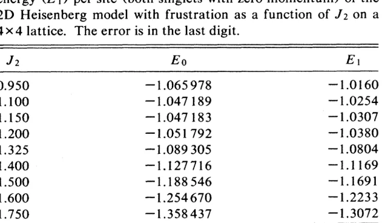
TABLE

I.

Ground-state energy

(Ep)

and first excited-state energy

(E~)

per site (both singlets with zero momentum)

of

the

2D Heisenberg model with frustration as a function

_{of J2}

on a

4X41attice.

The error is in the last digit.

ordered

(Neel)

disordered

(spin liquid?)

ordered

(¹el

in

each

sublattice)

FIG.

4.

(a)

Ground-state energy

(Eo)

and first excited-state

energy

(E~)

(per site) on a

4&4

lattice as a function

of

_Jz

near the degeneracy region. Also shown is the second excited-state

energy

(Ez).

The three states are singlets with

k=(0, 0).

For

comparison, we also show the triplet

(ET)

and singlet

(Es)

states

of

Fig.

2.

(b)

Possible phase diagram

of

the Heisenberg

model with frustration in the thermodynamic limit.

0.

950

1.

100

1.150

1.200

1.325

1.

400

1.

500

1.

600

1.750

Ep

—

_1.065

₉₇₈

—

_{1.047 189}

—

_{1.047 183}

—

_1.051

₇₉₂

—

_1.

₀₈₉

₃₀₅

—

_1.

₁₂₇

₇₁₆

—

_1.

_{188 546}

—

_1.

₂₅₄₆₇₀

—

_1.

₃₅₈₄₃₇

—

_1.

₀₁₆₀

—

_1.

₀₂₅₄

—

_1.

₀₃₀₇

—

_1.

₀₃₈₀

—

_1.

₀₈₀₄

—

_1.

₁₁₆₉

—

_1.1691

—

_1.2233

—

_1.3072

J

1-J2 Heisenberg model, Ns=4×4,

J1

=2.0

E. Dagotto and A. Moreo, PRB (R) 39 , 4744

(1989)

例題4: Kitaev model

1 0 0 1 0 5 1 2 0 13 1 6 0 4 0 2 1 5 1 3 0 12 0 6 1 13 1 7 0 10 0 14 1 11 1 15 3 2 2 3 2 1 3 4 2 15 3 8 2 0 2 4 3 1 3 5 2 14 2 8 3 15 3 9 2 6 2 16 3 7 3 17 5 4 4 5 4 3 5 0 4 17 5 10 4 2 4 0 5 3 5 1 4 16 4 10 5 17 5 11 4 8 4 12 5 9 5 13 7 6 6 7 6 11 7 8 6 1 7 12 6 10 6 8 7 11 7 9 6 0 6 12 7 1 7 13 6 16 6 2 7 17 7 3 9 8 8 9 8 7 9 10 8 3 9 14 8 6 8 10 9 7 9 11 8 2 8 14 9 3 9 15 8 12 8 4 9 13 9 5 11 10 10 11 10 9 11 6 10 5 11 16 10 8 10 6 11 9 11 7 10 4 10 16 11 5 11 17 10 14 10 0 11 15 11 1 13 12 12 13 12 17 13 14 12 7 13 0 12 16 12 14 13 17 13 15 12 6 12 0 13 7 13 1 12 4 12 8 13 5 13 9 15 14 14 15 14 13 15 16 14 9 15 2 14 12 14 16 15 13 15 17 14 8 14 2 15 9 15 3 14 0 14 10 15 1 15 11 17 16 16 17 16 15 17 12 16 11 17 4 16 14 16 12 17 15 17 13 16 10 16 4 17 11 17 5 16 2 16 6 17 3 17 7

is impossible, even if we introduce new terms in the Hamiltonian. On the other hand, the eight copies of each phase (corresponding to different sign combinations of Jx, Jy, Jz) have

the same translational properties. It is unknown whether the eight copies of the gapless phase are algebraically different.

We now consider the zeros of the spectrum that exist in the gapless phase. The momen-tum q is defined modulo the reciprocal lattice, i.e., it belongs to a torus. We represent the momentum space by the parallelogram spanned by (q1, q2)—the basis dual to (n1, n2). In

the symmetric case (Jx= Jy= Jz) the zeros of the spectrum are given by

ð34Þ If |Jx| and |Jy| decrease while |Jz| remains constant, q* and #q* move toward each other

(within the parallelogram) until they fuse and disappear. This happens when |Jx| + |Jy| = |Jz|. The points q*and #q*can also effectively fuse at opposite sides of the

par-allelogram. (Note that the equation q*= #q*has three nonzero solutions on the torus.)

At the points ±q*the spectrum has conic singularities (assuming that q*„ #q*)

ð35Þ

7. Properties of the gapped phases

In a gapped phase, spin correlations decay exponentially with distance, therefore spa-tially separated quasiparticles cannot interact directly. That is, a small displacement or another local action on one particle does not influence the other. However, the particles

J_x= =0J_z J_y= =0J_z =1, J_x J_y=1, =1, J_z J_x= =0J_y gapless gapped A_z A_x A_y B

Fig. 5. Phase diagram of the model. The triangle is the section of the positive octant (Jx, Jy, JzP 0) by the plane

Jx+ Jy+ Jz= 1. The diagrams for the other octants are similar.

20 A. Kitaev / Annals of Physics 321 (2006) 2–111

Annals of Physics 321, 2-111 (2016)

3方向のそれぞれが

Jx,Jy,Jzで相互作用

相図

可解模型→スピン液体

H =

J

x

X

x bond

S

_ix

S

_jx

J

y

X

y bond

S

_iy

S

_jy

J

z

X

z bond

S

_iz

S

_jz

lattice.gpで描画可能

例題4: Kitaev model

1. Lanczosでエネルギーを計算 (サイズ18サイト位)

2. TPQで比熱を計算: マヨラナ粒子の兆候がみえるか？

3. (発展)次近接のスピン相関が厳密に0を確認

4. (発展)ハイゼンベルク項をたすとどうなるか？

5. (発展)磁場をかけて磁化の温度依存性から帯磁率が計算可能

W = 3 L = 3 model = "SpinGC" method = "Lanczos" lattice = "Honeycomb" J0x = -1.0 J0y = 0.0 J0z = 0.0 J1x = 0.0 J1y = -1.0 J1z = 0.0 J2x = 0.0 J2y = 0.0 J2z = -1.0

H =

J

_x

X

x bond

S

_ix

S

_jx

J

_y

X

y bond

S

_iy

S

_jy

J

_z

X

z bond

S

_iz

S

_jz

例題5: Hubbard chain

H =

t

X

hi,ji

(c

†

_i

c

_j

+ h.c.) + U

X

i

n

_i

_"

n

_i

_#

L = 8

model = "FermionHubbard"

method = "Lanczos"

lattice = "chain"

t = 1.0

U = 8.0

nelec = 8

2Sz = 0

1. Lanczosでエネルギー・二重占有度を計算 (サイズ8サイト位)

2. TPQで比熱・二重占有度を計算:

3. (発展) 全対角化でアンサンブル平均を計算してTPQと比較

例題5: Hubbard chain (有限温度計算)

FullDiag, TPQ, Lanczosの比較

Hubbard model, L=8, U/t=8, half filling, S

z

=0

-0.5

0

0.5

1

1.5

2

2.5

0

0.05

0.1

0.15

0.2

0.25

10

-2

10

-1

10

0

10

1

10

2

10

-2

10

-1

10

0

10

1

10

2

D

/N

s

E

/N

s

TPQ

FullDiag

Lanczos

TPQ

FullDiag

Lanczos

T/t

T/t

3つの手法は互いに一致

その他の例

HPhi/samples/Standard/ 

に

_{Hubbard模型、Heisenberg模型、Kitaev模型、近藤格子模型}

の

_{Standard modeのStdFace.defがあります。}

StdFace.defを適宜変えて遊んでみてください。

注意：

-サイズは大きくし過ぎないこと

(PCだとspin 1/2で24site, Hubbardで12サイトくらいが限界)

-Lanczosはサイズが小さいと不安定です

(数千次元以上を推奨)

-TPQはサイズが小さいとうまくいきません

(数千次元以上を推奨)

物性研スパコンを使ってみよう!

物性研システムB (sekirei)

fat node: 1node (40 cores) 1TBのメモリ、

2nodesまで使用可 →

2TB

cpu node: 1node (24cores) 120GBのメモリ,

144nodesまで使用可 →

17TB

潤沢なメモリ: spin 1/2 36 sites, Hubbard 18 sitesまでなら

比較的簡単に計算可能 (5-10年程度前の最先端の計算)

TPQ法を使えば有限温度計算も可能！

お試しクラス(A) : 随時受付(100ポイント以下)

通常クラス(B,C,E): 年２回(6月,12月)受付

物性研スパコンを使ってみよう!

物性研システムB (sekirei)にはインストール済み

以下のようなスクリプトをサブミットするだけで、

大規模並列計算が可能

#!/bin/sh

#QSUB -queue F144cpu #QSUB -node 128 #QSUB -mpi 128 #QSUB -omp 24 #QSUB -place pack #QSUB -over false

#PBS -l walltime=24:00:00 #PBS -N HPhi

cd ${PBS_O_WORKDIR}

source /home/issp/materiapps/HPhi/HPhivars.sh

How to use HΦ: What is Expert mode ?

模型を指定するパラメーターファイル (3個)

zInterAll.def,zTrans.def, zlocspn.def

計算条件を指定するパラメーターファイル (2個)

modpara.def,calcmod.def

Standard mode:

計算に必要なファイルを

自動生成

相関関数を指定するパラメーターファイル (2個)

greenone.def, greentwo.def

HPhi -s StdFace.def

Expert mode

:計算に必要なファイルを

自分で用意

→Standard modeで生成したものを書き換えるのが楽

+ファイル名を列挙したファイル: namelist.def

How to use HΦ: What is Expert mode ?

HPhi

-e

namelist.def

Expert mode

:計算に必要な以下のファイルを

自分で用意

→Standard modeで生成したものを書き換えるのが楽

用意して以下のコマンドを実行

模型を指定するパラメーターファイル (3個)

zInterAll.def,zTrans.def, zlocspn.def

計算条件を指定するパラメーターファイル (2個)

modpara.def,calcmod.def

相関関数を指定するパラメーターファイル (2個)

greenone.def, greentwo.def

How to use HΦ: zInterall.def

「任意」の2体の相互作用を指定することができる

(自動生成するようにしておくと便利)

→任意の格子を指定することが出来る

模型を指定するパラメーターファイルの例

相互作用の総数

実部

虚部

i σ

1

j σ

2

k σ

3

l σ

4

H+ =

X

i,j,k,l

X

1, 2, 3, 4

I

_{ijkl 1 2 3 4}

c

†_{i 1}

c

_{j 2}

c

†_{k 3}

c

_{l 4}

How to use HΦ: Expert mode

模型を指定する簡易版のパラメータファイル

- CoulombIntra

-Exchange

4.2

エキスパートモード用入力ファイル

49

4.2.7

CoulombIntra

指定ファイル

オンサイトクーロン相互作用をハミルトニアンに付け加えます

(S = 1/2

の系で

のみ使用可能、

ver. 0.2

では

MPI

非対応

)

。付け加える項は以下で与えられます。

H+ =

!

i

U

i

n

i_↑

n

i_↓

(4.12)

以下にファイル例を記載します。

✓

✏

======================

NCoulombIntra 6

======================

========i_0LocSpn_1IteElc ======

======================

0

4.000000

1

4.000000

2

4.000000

3

4.000000

4

4.000000

5

4.000000

✒

✑

ファイル形式

以下のように行数に応じ異なる形式をとります。

• 1

行

:

ヘッダ

(

何が書かれても問題ありません

)

。

• 2

行

: [string01] [int01]

• 3-5

行

:

ヘッダ

(

何が書かれても問題ありません

)

。

• 6

行以降

: [int02] [double01]

パラメータ

• [string01]

形式

: string

型

(

空白不可

)

説明

:

オンサイトクーロン相互作用の総数のキーワード名を指定します

(

任意

)

。

• [int01]

形式

: int

型

(

空白不可

)

説明

:

オンサイトクーロン相互作用の総数を指定します。

• [int02]

形式

: int

型

(

空白不可

)

説明

:

サイト番号を指定する整数。

0

以上

Nsite

未満で指定します。

4.2

エキスパートモード用入力ファイル

57

4.2.11

Exchange

指定ファイル

Exchange

カップリングをハミルトニアンに付け加えます

(S = 1/2

の系でのみ

使用可能、

ver. 0.2

では

MPI

非対応

)

。電子系の場合には

H+ =

!

i,j

J

_ijEx

(c

†_i↑

c

_j↑

c

†_j↓

c

_i↓

+ c

†_i↓

c

_j↓

c

†_j↑

c

_i↑

)

(4.16)

が付け加えられ、スピン系の場合には

H+ =

!

i,j

J

_ijEx

(S

_i+

S

_j−

+ S

_i−

S

_j+

)

(4.17)

が付け加えられます。スピン系の

(S

_i+

S

_j−

+ S

_i−

S

_j+

)

を電子系の演算子で書き直すと、

−(c

†i_↑

c

j↑

c

†j_↓

c

i↓

+ c

†i_↓

c

j↓

c

†j_↑

c

i↑

)

となることに注意して下さい。以下にファイル例を記載

します。

✓

✏

======================

NExchange 6

======================

========Exchange ======

======================

0

1

0.50000

1

2

0.50000

2

3

0.50000

3

4

0.50000

4

5

0.50000

5

0

0.50000

✒

✑

ファイル形式

以下のように行数に応じ異なる形式をとります。

• 1

行

:

ヘッダ

(

何が書かれても問題ありません

)

。

• 2

行

: [string01] [int01]

• 3-5

行

:

ヘッダ

(

何が書かれても問題ありません

)

。

• 6

行以降

: [int02] [int03] [double01]

パラメータ

• [string01]

形式

: string

型

(

空白不可

)

説明

: Exchange

カップリングの総数のキーワード名を指定します

(

任意

)

。

================================= NExchange 2 ================================= ===========Exchange============== ================================= 0 1 0.5 1 2 0.5 ================================= NCoulombintra 2 ================================= ===========Exchange============== ================================= 0 4.0 1 4.0

指定が楽&高速化することも

詳細はマニュアル参照

HΦを使いこなすには..

- 簡単なファイルの書き出し、読み込み&解析が

できると計算後の解析の幅が格段に拡がります

-もちろん、通常のプログラミング言語(fortran, C++/Cなど)

でも十分できますが、

スクリプト言語(python, perl, rubyなど)を覚えて

おくと便利です。sed、awkといったコマンドを

使うのも楽ですが、拡張性が低いのが難点です

-自分で気に入ったものを使うのが一番ですが、

周りに詳しい人がいる言語を選択するのが無難でしょうか..

-計算物質科学の分野だと主流はpythonでしょうか..

あとはやりたいこと

をやってください

- 近藤格子模型

- カゴメ格子,三角格子…

解析したい模型などの

相談・質問も大歓迎です!