A simple procedure to approximate slip displacement of freestanding rigid body subjected to earthquake motions

A SIMPLE PROCEDURE TO APPROXIMATE SLIP DISPLACEMENT OF FREESTANDING RIGID BODY SUBJECTED TO EARTHQUAKE MOTIONS

Tomoyo TANIGUCHI1 and Takuya MIWA2

1 _{Associate Professor, Department of Civil Engineering, Tottori University. 4-101 Koyama-Minami Tottori,}

680-8552, Japan. Tel +81-857-31-5287, Fax +81-857-28-7899, Email: [email protected]

2 _{Engineer, Bridge Design Department, TTK Corporation. 1020 Ooaza-Simotakai, Toride, 302-0038, Japan. Tel}

+81-297-78-1119, Fax +81-0297-78-5344, Email: [email protected] (Former graduate student, Department of Civil Engineering., Tottori University)

SUMMARY

A simple calculation procedure for estimating absolute maximum slip displacement of a freestanding rigid body placed on the ground or floor of linear/nonlinear multi-story building during an earthquake is developed. The proposed procedure uses the displacement induced by the horizontal sinusoidal acceleration to approximate the absolute maximum slip displacement, i.e., the basic slip displacement. The amplitude of this horizontal sinusoidal acceleration is identical to either the peak horizontal ground acceleration or peak horizontal floor response acceleration. Its period meets the predominant period of the horizontal acceleration employed. The effects of vertical acceleration are considered to reduce the friction force monotonously. The root mean square value of the vertical acceleration at the peak horizontal acceleration is used. A mathematical solution of the basic slip displacement is presented. Employing over one hundred accelerograms, the absolute maximum slip displacements are computed and compared with the corresponding basic slip displacements. Their discrepancies are modeled by the logarithmic normal distribution regardless of the analytical conditions. The modification factor to the basic slip displacement is quantified based on the probability of the nonexceedence of a certain threshold. Therefore, the product of the modification factor and the basic slip displacement gives the design slip displacement of the body as the maximum expected value. Since the place of the body and linear/nonlinear state of building make the modification factor slightly vary, ensuring it to suit the problem is essential to secure prediction accuracy.

Keywords; horizontal sinusoidal acceleration, maximum expected slip displacement, coincident vertical

acceleration, predominant period, peak horizontal ground acceleration, peak horizontal floor response acceleration.

INTRODUCTION

In recent highly developed and complicated social system the damage of structures no longer represents total effects of earthquakes. The functional loss of the social system as a result of the damage of nonstructural component should be taken into account. An appropriate design for nonstructural components to maintain minimum function in the event of earthquakes prevents from such systematic disorder. The former investigators clearly pointed out a need for investigation into seismic behavior of nonstructural components in order to assess

their vulnerability [1]. An important class of nonstructural components, such as mechanical/electrical equipment, which is essentially modeled as a rigid body, is of interest to this study.

The effects of base excitation on a freestanding rigid body have been investigated by many researchers. They clarified five modes of the body (rest, slide, rock, slid-rock and jump), equations of motion and relation of wave properties of base excitation to these modes [2-6]. The senior author pointed out that the period of horizontal base excitation makes an important contribution to elongation of the slip displacement of the body in addition to the friction coefficient and peak horizontal acceleration [7].

Shao and Tung [8] prepared a chart which enabled to determine the mean-plus-standard deviation of the maximum sliding distance of an unanchored body. However, the study does not consider vertical excitation and its applicability to the body placed on the building floor. Including the vertical excitation, Lopez Garcia and Soong [1] presented the fragility information for sliding related failure modes. They classified the fragility curves according to the friction coefficient and peak horizontal ground acceleration. Although it gives the appropriate slip displacement if the body is on the ground, its prediction accuracy deteriorates when the body is on the building floor. Historically, Newmark [9] presented a simple formula to determine the sliding distance of a freestanding body subjected to a single rectangular acceleration pulse at the base concerning earthquake response of embankments. Choi and Tung [10] concluded that Newmark’s formula could be used if an adjustment factor consisting of the friction coefficient and peak horizontal base acceleration was applied. However, the study is limited to the action of horizontal base excitation. In addition to that, prediction accuracy deteriorates if the body is on the building floor with a long natural period.

As mentioned above, the previous procedures for estimating the slip displacement of the body do not consider the period of horizontal excitation. Consequently, the prediction accuracy of the slip displacement of the body on the building floor may deteriorate because filtering effects of structure enhance the advent of a certain wave component in the floor response. This suggests the necessity of considering the period of horizontal excitation to approximate the slip displacement of the body set on the building floor.

An objective of this study is to develop a simple procedure that can approximate the absolute maximum slip displacement of the body during the earthquake wherever it is set on, i.e., the design slip displacement. In order to improve the deficiencies in the previous research, this study introduces the use of the single horizontal sinusoidal acceleration. Its amplitude is identical to either the peak horizontal ground acceleration or the peak horizontal floor response acceleration. Its period meets the predominant period of the horizontal acceleration employed. Generally, the peak horizontal ground acceleration is not always induced by the wave component with the predominant period of earthquake. On the other hand, due to filtering effects of structure, the peak horizontal floor response acceleration tends to be induced by the wave component with the predominant period of floor response. This is the advantage of the use of the horizontal sinusoidal acceleration.

The slip displacement of the body induced by the horizontal sinusoidal acceleration, i.e., the basic slip displacement, is used as the first approximation to the absolute maximum slip displacement of the body, since it

gives an upper bound of the slip displacement under the single action of horizontal base acceleration. The discrepancy between the basic slip displacement and absolute maximum slip displacement are compiled to find the modification factor for the basic slip displacement. Since it is statistically examined based on the probability of nonexceedence of a certain threshold, the design slip displacement is given as the maximum expected value. In contrast, Shao and Tung [8] suggested that the effects of the vertical ground motion on the mean-plus-standard deviation of the maximum sliding distance was small but it was indispensable to compute the slip displacement of the body accurately. In view of developing a simple calculation procedure and having a safety margin in slip displacement, this study introduces a monotonous reduction in friction force as if the uniform downward acceleration lasts while the body slips under action of the horizontal sinusoidal acceleration. The use of the root mean square value of the vertical acceleration at the peak horizontal acceleration [11, 12] is proposed as the uniform downward acceleration.

The fist part of the paper briefly describes the problem and the second part defines the horizontal sinusoidal acceleration and derives a mathematical solution of the basic slip displacement. The third and forth part examines the modification factor for the basic slip displacement of the body set on the ground and the building floor respectively. Three buildings with different stories and spans and liner/nonlinear state are considered.

DESCRIPTION OF THE PROBLEM

An equation of motion that governs the slip behavior of the body subjected to simultaneous horizontal and vertical acceleration is given as follows. Figure 1(a) and Figure 1(b) shows a mechanical model of the body placed on the ground and set on the building floor respectively. If we replace the shaking motion according to the problem, the subjects are essentially the same.

i) while slip x&&=−z&&_h−ν(g+z&&_v)sign

( )

ii) while stationary x&&=0 (2)

iii) slip commencement condition z&&_h >μ(g+z&&_v) (3)

iv) slip termination condition x&=0 (4)

where and are a pair of horizontal and vertical acceleration of either the ground or building floor,

respectively. h

z&& z&&v

g, μ and ν are gravitational acceleration, static and kinetic friction coefficients, respectively. In

order to simplify the problem, the static and kinetic friction coefficients are assumed to be the same and denoted

as μ thereafter. The function sign &

( )

BASIC SLIP DISPLACEMENT OF THE BODY Simplification of the problem

A simple treatment of the vertical acceleration is necessary to mathematically obtain the slip displacement of the body induced by the horizontal sinusoidal acceleration, i.e., the basic slip displacement of the body. Employing Eqs. (1) to (4) and all accelerograms listed on Table 1, the absolute maximum slip displacement of the body with/without the vertical ground acceleration is numerically computed. Each pair of horizontal and vertical

assumed to be 0.3 to 0.5. The abscissa of Figure 1(c) is the ratio of the slip displacement induced by the simultaneous horizontal and vertical ground acceleration to the slip displacement induced by horizontal ground acceleration. The ordinate is the probability density of the frequency. Although the vertical ground acceleration does not always increase the slip displacement, it is better to ensure an adequate safety margin against the slip displacement. Since the slip motion of the body discontinuously occurs during the earthquake and lasts a short time, the effects of varying vertical acceleration on the slip motion of the body have few contributions. Therefore, this study introduces a monotonous reduction in friction force while the body slips [13]. To calculate the basic slip displacement of the body, Eqs. (1) and (3) are rewritten as follows.

( )

z

x&&=−&&h−μ( −σ⋅ ⋅η) & (5) )

PVGA g

(

z&&_h >μ −σ⋅ ⋅η (6)

where is the horizontal sinusoidal acceleration defined by Eq. (7). z&&_h σ is the standard deviation of the ratio of

the vertical ground acceleration to the peak vertical ground acceleration (PVGA) at the instant of PHGA. The senior author(s) compiled this ratio with 144 accelerograms. The probability density of this ratio was modeled by

the normal distribution and the product of σ and PVGA gave the root mean square value of the vertical ground

acceleration. A pair of this vertical ground acceleration and PHGA was used for verification of the onset of slip of the unanchored flat-bottom cylindrical shell tank [11]. In addition, the probability density of this ratio computed with the ground acceleration was almost the same as that computed with the building floor response

acceleration [12]. Therefore, this paper uses 0.46 as the value of σ irrespective of the location of the body

placed on. In case of the body set on the ground, this paper uses PVGA of each vertical accelerogram. In actual case scenario, although the value of PVGA is usually not provided by design codes, it can be determined by the

ratio of PVGA to PHGA [14] or the well-known empirical rule PVGA = 0.5 or 0.66 PHGA. In contrast, η is the

magnification factor for the vertical floor response given by the quotient of the peak vertical floor response acceleration (VFRA) by PVGA. This paper uses the peak VFRA of each result of time history analysis as the

value of PVGA⋅η. In actual case scenario, η is determined by the response amplitude. Therefore, η is 1.0 if the

body is set on the ground.

Horizontal sinusoidal acceleration

The amplitude of the horizontal sinusoidal acceleration, , is identical to PHGA if the body is placed on the

ground. In contrast, it should be identical to the peak horizontal floor response acceleration (HFRA) if the body is set on the building floor.

g A_gx ⎟ ⎠ ⎞ ⎜ ⎝ ⎛ = t T g A z&&_{h gx} sin 2π (7)

where is the predominant period of the horizontal acceleration (PPHA) of either the horizontal ground

acceleration or floor response acceleration. In case of the body set on the ground, this paper uses PPHA determined by the period which maximizes a pseudo-acceleration spectrum of each horizontal accelerogram. In actual case scenario, PPHA is determined by the natural period of soil, since it will be predominant over other

wave period in the earthquake. Ref. [14] gives the calculation of the natural period of soil. In case of the body set on building floor, this paper uses PPHA determined by FFT analysis of each horizontal floor acceleration. For the convenience of actual case scenario, the calculation of the predominant period of the horizontal floor response acceleration is proposed latter.

Mathematical solution

Solve Eqs. (5) to (7) mathematically to obtain the basic slip displacement of the body. Firstly, assume an absence of the vertical acceleration to simplify the problem. Figures 1(d) and 1(e) depict the typical time history of slip

motion of the body subjected to the horizontal sinusoidal acceleration with A_gx g=7m/s2, T=6.28s and μ=0.4.

When the body undergoes the horizontal base acceleration, the body begins to slip when the horizontal inertia

force overcomes the friction force. From Eqs. (6) and (7), the time, , for the onset of slip is calculated as: t0

gx A Sin T t μ π 1 0 ₂ − = (8)

Despite the time history of horizontal base acceleration the slip acceleration of the body is uniform. The velocity of the body at arbitrary time is calculated as:

x&=μgt+C1 (9)

Similarly, the velocity of the base is calculated as:

t T T g A zh gx π π 2 cos 2 − = & (10)

where the initial velocity of the base is assumed to be −A_gx gT 2π to derive Eq. (10). In contrast, in Eq. (9) is

the constant of integration and should be determined as that the body has the same velocity of the base at the onset of slip. 1 C ⎟ ⎟ ⎠ ⎞ ⎜ ⎜ ⎝ ⎛ ⎟ ⎟ ⎠ ⎞ ⎜ ⎜ ⎝ ⎛ + − = − − gx gx gx A Sin g A A gSin T C μ μ μ π 1 1 1 cos 2 (11)

From Fig. 1(e), the slip terminates when the velocity of the body and base become the same. The time is calculated by Eqs. (9), (10) and (11) as follows.

t T T g A A Sin g A A Sin g T gt _gx gx gx gx π π μ μ μ π μ cos2 2 cos 2 1 1 ₌₋ ⎟ ⎟ ⎠ ⎞ ⎜ ⎜ ⎝ ⎛ ⎟ ⎟ ⎠ ⎞ ⎜ ⎜ ⎝ ⎛ + − − − ₍₁₂₎

Solve Eq. (12) for t to find the slip termination time, . Since Eq. (12) is, however, the transcendental function

in terms of the cosine function, this study tries to find its approximate solution employing the Taylor’s series.

From Figs. 1(d) and 1(e), since the slip terminates around t=

1

t

2

T , the Taylor’s series of the cosine function

around t=T 2 is used. L 2 2 2 2 2 1 2 cos ⎟ ⎠ ⎞ ⎜ ⎝ ⎛ − + − ≈ t T T t T π π ₍₁₃₎

⎟⎟ ⎟ ⎠ ⎞ ⎜⎜ ⎜ ⎝ ⎛ ⎪⎭ ⎪ ⎬ ⎫ ⎪⎩ ⎪ ⎨ ⎧ ⎟⎟ ⎠ ⎞ ⎜⎜ ⎝ ⎛ − + + + − = 2 1 2 2 2 2 1 π φ ϕ ϕ π gx gx gx A A A T t , where ϕ =μ−πAgx, ⎟⎟ ⎠ ⎞ ⎜ ⎜ ⎝ ⎛ + = − − gx gx gx A Sin A A Sin μ μ μ φ 1 _cos 1 ₍₁₄₎

Therefore, the basic slip displacement,

,

the duration of the slip.

Sin h x 2 1 11 2 2 2 1 2 sin 4 2 1 2 sin 1 0 1 0 D t D t T gT A μgt dtdt t T π g A μg x t gx t t t gx Sin h ⎟ = + + + ⎠ ⎞ ⎜ ⎝ ⎛ ₋ =

_{∫ ∫}

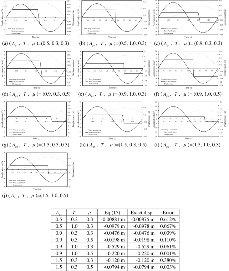
It is worth nothing that and are determined by only parameters that specify the slip motion of the body. Figures 2(a) to 2(j) show the slip motion of the body induced by the sinusoidal base acceleration. The title of

each figure shows a combination of analytical condition = 0.5 to 1.5, T= 0.3 to 1.0 and

0

t t1

gx

A μ= 0.3 to 0.5.

Although the slip termination time varies t=5T 8 to 3T 4 with the change in the analytical condition, Eq. (15)

well approximates the exact slip displacement computed numerically (See Figure 2(k)). Since the value of the cosine function increases monotonously in the range considered herein, the Taylor’s series of the cosine function

around t=T 2favorably works.

Finally, consider the action of the monotonous downward vertical acceleration. Simply replacing the friction

coefficient, μ , of Eqs. (8) to (15) by the nominal friction coefficent μ′=μ

(

)

displacement Sin is calculated by the same manner.

v h

x_,

DESIGN SLIP DISPLACEMNT OF THE BODY ON THE GROUND Methodologies

Although the horizontal sinusoidal acceleration possesses representative characters of the earthquake wave, it does not include all properties that randomly appear in the earthquake wave. Therefore, the basic slip displacement is naturally different from the absolute maximum slip displacement induced by the earthquake. This paper considers it as the estimation error of the proposed procedure since the basic slip displacement is deterministically calculated while the absolute maximum slip displacement is influenced by the randomness of the earthquake wave. The discrepancies between them are compiled. The modification factor for the basic slip displacement to calculate the design slip displacement is statistically examined.

Earthquake records

This study uses 104 accelerograms observed around Japan [15]. The slip displacement discussed herein is inevitably affected by regional properties of accelerogram samples, although these earthquakes are of different characteristics in terms of energy content in various frequency bands, duration, and variation of intensity with respect to time (See Table 1). According to the classification of soil type on Ref. [14], the natural period of hard soil is less than 0.2 s, that of soft soil is longer than 0.6 s, and remaining is classified as the medium soil. Each soil type has 34, 42, and 28 accelerograms, respectively. The time history of horizontal acceleration is first

normalized. That is, for each acclelerogram, PHGA is scaled to a value of g. When one is interested in the

statistics of the slip displacement of a body to say, 0.4 g, other than g, all horizontal acceleration time histories

are scaled by multiplying them by the value of 0.4. Maintaining the relation between PHGA and PVGA of each pair of accelerograms, the time history of vertical acceleration is also normalized and scaled in a same manner. Employing a pair of scaled accelerograms in and , the time history of slip displacement is numerically computed by ACSL with 0.001 seconds intervals [16].

h z&& z&&v

Modification factor for basic slip displacement

The absolute maximum slip displacement of the body induced by the earthquake wave,

Max Eq

v h

x_, , is numerically

computed and compared with the corresponding basic slip displacement, , induced by the horizontal

sinusoidal acceleration with the nominal friction coefficient, μ

Sin v h

x,

′. Introducing the slip ratio, β_h,v, the estimation

errors are statistically examined.

Sin v h Max Eq v h v h x x , , , = β (16)

There are three primary reasons that the basic slip displacement is different from the absolute maximum slip displacement.

1) The wave form of earthquake is different from that of the horizontal sinusoidal acceleration while the body slips.

2) The wave period of earthquake is different from that of the horizontal sinusoidal acceleration while the body slips.

3) Since the wave of earthquake is naturally asymmetric, the slip displacement is sometimes one-sided.

Since these are general characteristics of estimation errors and interpreted accordingly, the modification factor for the basic displacement to approximate the absolute maximum slip displacement is statistically defined.

Figures 3(a) to 3(c) show the probability density of the slip ratio, . The slip ratio is classified according to a

combination of PHGA and μ. The legend in each figure shows the value of μ. PHGA and friction coefficient are assumed to be 5m/s

v h, β

2 _{to 9m/s}2 _{and 0.3 to 0.5 respectively. From these figures, the slip ratio, , possesses}

almost the same probability density irrespective of the combination of PHGA and μ. Figure 3(d) shows the

probability density of the slip ratio, , classified according to the soil type without identification of PHGA and

μ. The slip ratio, , also possesses almost the same probability density irrespective of soil types.

Consequently, the probability density of the slip ratio, , is compiled irrespective of analytical conditions.

Figure 3(e) shows the probability density of the slip ratio,

v h, β v h, β v h, β v h, β v h,

β , of all results. The distribution is modeled by the

logarithmic normal distribution function whose mean and standard deviation are 0.83 and 0.78 respectively. The

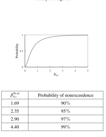
solid line in Figure 3(e) presents an approximation. Figure 4 shows the probability of the slip ratio β_h,v

converted from Figure 3(e). A table below the figure shows the value of the modification factor, , for the

selected probability of the nonexceedence of the specified threshold. The product of the modification factor,

ob v h

βPr ,

ob v h

βPr

, , and the basic slip displacement,

,

,

value. Sin v h x_, Exp v h x_, (17) Sin v h ob v h Exp v h x x Pr _, , , =β ⋅

Here, in the absence of vertical ground motion, our previous study revealed that the mean and standard deviation of the slip ratio were 1.03 and 0.71, respectively [13]. Having the value of 1.03 in the mean suggests that the largest slip displacement is likely induced by the wave with PPHA and corroborates the importance of consideration of PPHA. However, the monotonous reduction in friction force slightly overestimates the effects of the vertical ground acceleration on the slip displacement of the body as a consequence of that the inclusion of vertical ground motion decreases the mean 19%. In contrast, since these standard deviations are the same order, the proposed procedure maintains the estimation accuracy if the vertical ground acceleration is considered.

DESIGN SLIP DISPLACEMNT OF THE BODY ON THE BUILDING FLOOR Methodologies

The following section tries to apply the proposed procedure to estimate the slip displacement of the body set on the building floor. All parameters that define the horizontal sinusoidal acceleration, i.e., PHGA, PVGA and PPHA, should be replaced by the peak HFRA, peak VFRA and corresponding PPHA, respectively. The absolute maximum slip displacement of the body induced by the floor response acceleration is compapred with the corresponding basic slip displacement. The modification factor for the basic slip displacement is statistically examined.

Time history of floor response

This investigation uses three actual concrete building models with different stories and spans and 3% structural damping illustrated in Figure 5(a). The dimensions of each column and beam are shown in Figure 5(b). Figure 5(c) shows the natural period of each mode of each building. PHGA of all accelerograms listed in Table 1 is scaled to 250gal for linear analysis and 500gal for nonlinear analysis. In nonlinear analysis, all columns maintain elasticity, while plastic hinges appear on beams at beam-column connections. The nonlinear property of the beam is modeled by Takeda-model [17]. The time history of HFRA and VFRA are picked up at top and middle floors of each building. The dynamic analysis of building is carried out by commercial software TDAP III [17] without a contribution to slip of the body. Since the nonlinear model of the beam affects the properties of floor response, the nature of slip behavior at other type of nonlinear model differs from that observed herein. Since it affects the statistical properties of the slip ratio, the other slip ratio is necessary for the case.

Predominant period of horizontal floor response acceleration

To know the predominant period of HFRA is essential to secure the prediction accuracy of the slip displacement of the body set on the building floor. Strictly speaking, we need to know the predominant period of HFRA that causes the largest slip displacement in the time history because it dominates the absolute maximum slip displacement of the body, i.e., dominant slip displacement. In most cases, this HFRA is identical to the peak HFRA. Therefore, picking up the HFRA for three seconds around the onset of the dominant slip displacement,

the component of wave period is investigated by FFT analysis. To find typical characters in the predominant period of HFRA, the following investigation uses twenty accelerograms randomly chosen from Table 1. Figures 6(a) to 6(c) show the predominant period of HFRA observed at the specified floor of linear building while Figures 6(d) to 6(f) show that of nonlinear building. The abscissa of these figures shows the predominant period of earthquake input to the building model determined by a pseudo-acceleration spectrum of each earthquake. The ordinate of these figures shows the predominant period of HFRA that causes the dominant slip displacement. The horizontal lines in each figure show the natural period of the first three modes of each building. From these figures, the following typical characteristics are found [18].

1) The predominat period of HFRA is close to that of horizontal ground acceleration if the nonlinearity of structure appears before HFRA reaches its peak (See Group 1 in Figures 6(d) to 6(f)). Since the nonlinearity of structure diminishes filtering effects of structure, properties of earthquake wave appear directly on the floor response.

2) The predominant period of HFRA is not close to that of horizontal ground acceleration when the structure keeps elasticity or just reaches nonlinear region at an instant of the peak HFRA (See Figures 6(a) to 6(c) and Group 2 in Figures 6(d) to 6(f)). However, the predominant period of HFRA is not always identical to either the natural period of modes of structure, since the structure is always in transient response during an earhtquake. It implies the necessity of developing an estimation method of the predominant period of HFRA. This paper attemps to predict the predominant period of HFRA by superposing the natural period of each mode inspired from the root mean square method.

Figures 6(g) to 6(i) examine the prediction accuracy of the predominant period of HFRA with all acclerograms, floor loction, building types and linear/nonlinear state of building. The proposed method can adequately predict the predominant period of HFRA despite the analytical conditions.

Modification factor for basic slip displacement (buildings in linear state)

Firstly, consider the buildings in linear state. The absolute maximum slip displacement of the body induced by HFRA and VFRA,

Max Fl

v h

x_, , is numerically computed and compared with the corresponding basic slip

displacement, Sin, induced by the horizontal sinusoidal acceleration with the nominal friction coefficient, μ

v h

x_, ′.

Introducing the slip ratio, βh,v, the estimation errors are statistically examined.

Sin v h Max Fl v h v h x x , , , = β (18)

Figures 7(a) to 7(f) show the probability density of the slip ratio, β_h,v, classified according to the floor location,

building type and μ. Similar to, , observed on the ground, the slip ratio, , forms a certain probability

density despite the analytical conditions. Figure 7(g) is the probability density of the slip ratio,

v h, β β_h,v v h, β , of all

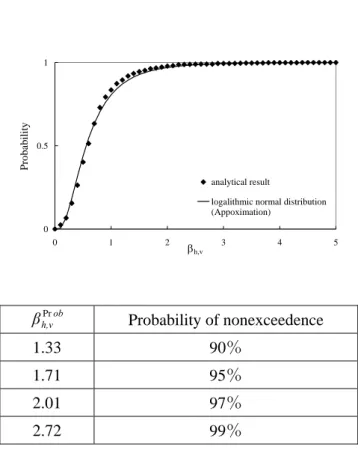
results. The distribution is modeled by the logarithmic normal distribution function whose mean and standard deviation are 0.70 and 0.54, respectively. The solid line in Figure 7(g) presents an approximation. Figure 8

shows the probability of the slip ratio, β_h,v, converted from Figure 7(g). A table below the figure shows the

value of modification factor, , for the selected probability of the nonexceedance of the specified threshold.

Employing Eq. (17), the design slip displacement,

,

, and the basic slip displacement, .This simplification imposes restriction on the proposed method. For

instance, adoption of the unique value of

ob v hPr, β Exp v h x, ob v hPr, β Sin v h x, v h,

β in estimating the slip displacement of the body set on the first floor

where the filtering effects of structure cannot be expected leads considerable error.

A comparison of Figures 3(e) and 7(g) yields advantage of the use of the horizontal sinusoidal acceleration since the standard deviation of Figure 7(g) is 69% of that of Figure 3(e). The inherent randomness in the earthquake is diminished by filtering effects of structure and the wave form of HFRA becomes similar to that of the horizontal sinusoidal acceleration. In contrast, in addition to overestimation of effects of the vertical ground acceleration, decrease in the mean is caused by the estimation error of the predominant period of HFRA because the proposed method tends to estimate the predominant period of HFRA to be slightly longer. Therefore, ensuring the modification factor to suit the problem is essential to secure the prediction accuracy of the slip displacement.

Modification factor for basic slip displacement (buildings in nonlinear state)

Secondly, consider the buildings in nonlinear state. Employing Eq. (18), the slip ratio, β_h,v, is statistically

examined.

Figures 9(a) to 9(f) show the probability density of the slip ratio, βh,v, classified according to the floor location,

building type and μ. Similar to previous discussion, the slip ratio forms a certain probability density despite

the analytical conditions. Figure 9(g) shows the probability density of the slip ratio

v h, β

v h,

β of all results. The

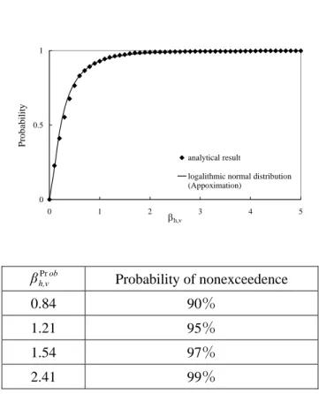
distribution is modeled by the logarithmic normal distribution function whose mean and standard deviation are 0.38 and 0.51 respectively. The solid line in Figure 9(g) presents an approximation. Figure 10 shows the

probability of the slip ratio, , converted from Figure 9(g). A table below the figure shows the value of

modification factor, , for the selected probability of the nonexceedance of the specified threshold.

Employing Eq. (17), the design slip displacement,

,

, and the basic slip displacement, .

v h, β ob v h Pr , β Exp v h x_, ob v h Pr , β Sin v h x_,

From Figures 7(g) and 9(g), the prediction accuracy slightly deteriorates since the mean decreases 46% but the standard deviation maintains the same order. In addition to the overestimation of effects of the vertical ground acceleration, decrease in the mean is caused by the dissimilarity of the wave form between HFRA of the building in the nonlinear state and the horizontal sinusoidal acceleration [18]. Figure 11(a) shows the time history of HFRA and slip acceleration of the body observed at linear building. Figure 11(b) magnifies the onset of the dominant slip displacement. The approximation of the floor motion by the horizontal sinusoidal acceleration is also plotted. The similarity between HFRA and the horizontal sinusoidal acceleration and slip acceleration induced by them corroborates the applicability of the proposed procedure. In contrast, Figures 11(c) and 11(d) show those observed at nonlinear building. The dissimilarity between HFRA and the horizontal sinusoidal acceleration and its effects on the slip acceleration can be seen. The advantage of the use of the sinusoidal wave

slightly diminishes. However, since these standard deviations still keep the same order, the proposed procedure maintains the estimation accuracy if the nonlinearity of the structure is considered. Therefore, ensuring an adequate modification factor to suit the problem is essential to secure the prediction accuracy of the slip displacement.

CONCLUSION

This paper proposes the use of the horizontal sinusoidal acceleration to approximate the slip displacement of the body wherever it is set on during an earthquake. A mathematical solution of the slip displacement of the body induced by the horizontal sinusoidal acceleration, i.e., the basic slip displacement, is presented in a practical form. The product of the basic slip displacement and the modification factor gives the design slip displacement as the maximum expected value. The modification factor is quantified as an estimation error between the basic slip displacement and the absolute maximum slip displacement based on the probability of the nonexceedence of a certain threshold. It forms a certain probability density despite the acceleration intensity and the friction coefficient. However, the modification factors are slightly different according to the place of the body and linear/nonlinear state of building. In order to secure the prediction accuracy of the slip displacement of the body, ensuring the modification factor to suit the problem is essential.

REFERENCES

1. Lopez Garcia D, Soong TT. Sliding fragility of block-type non-structural components, Part I: unrestrained

components, Earthquake Engineering and Structural Dynamics 2003; 32(1): 111-129.

2. Ishiyama Y. Motions of rigid bodies and criteria for overturning by earthquake excitations. Earthquake

Engineering and Structural Dynamics 1982; 10: 635-650.

3. Shenton III HW, Jones NP. Base excitation of rigid bodies. I: formulation. Journal of Engineering

Mechanics, ASCE, 1991; 117: 2286-2306.

4. Shenton HW III. Criteria for initiation of slide, rock, and slide-rock rigid-body modes. Journal of

Engineering Mechanics, ASCE, 1996; 122(7): 690-693.

5. Taniguchi T and Murayama T. Study of free liftoff induced slip behavior of rectangular rigid bodies. PVP,

Seismic Engineering, ASME, 2001: 428-1: 123-130.

6. Taniguchi T. Experimental and analytical study of free lift-off motion induced slip behavior of rectangular

rigid bodies. Journal of Pressure Vessel Technologies, ASME, 2004: 126(1): 53-58.

7. Taniguchi T. Nonlinear response analyses of rectangular rigid bodies subjected to horizontal and vertical

ground motion. Earthquake Engineering and Structural Dynamics, 2002; 31: 1481-1500.

8. Shao Y, Tung CC. Seismic response of unanchored bodies. Earthquake Spectra, 1999; 15(3): 523-536.

9. Newmark NM. Effects of earthquakes on dams and embankments, Geotechnique, 1965; 15(2): 139-160.

10. Choi B, Tung CC. Estimating sliding displacement of an unanchored body subjected to earthquake excitation. Earthquake Spectra, 2002; 18(4): 601-613.

flat-bottom cylindrical shell tank subjected to horizontal and vertical ground motion. Journal of Structural Mechanics and Earthquake Engineering, JSCE, 2000; 611(I-53): 95-105 (Japanese).

12. Taniguchi T, Takeshita M. Coincident vertical response analysis of structure at maximum horizontal response. 13WCEE, No.433, 2004.

13. Taniguchi T, Miwa T. Slip displacement analysis of freestanding rigid bodies subjected to earthquake motions. 13WCEE, No.437, 2004.

14. Japan Road Association. Specifications for Highway Bridges-Part V: Seismic Design. 2002 (Japanese). 15. National Information Center for Earthquakes and Disasters, http://www.bosai.go.jp/

16. ACSL Reference Manual; Edition 11.1, MGA Software: Concord, 1995. 17. TDAP III ver.2.11.01. ARK Information Systems, 2002.

18. Miwa T. A study of slip displacement of rigid body considering period of shaking. Mater thesis, Tottori University, 2004 (Japanese)

Tomoyo Taniguchi

Table 1 List of accelerograms

Name of Earthquake PHGA(gal) PVGA(gal) PPHA(s) Name of Earthquake PHGA(gal) PVGA(gal) PPHA(s)

aic0160401061450 53.303 15.661 0.288 myz0099610192344 31.052 16.220 0.8 aic0169703161451 109.096 29.596 0.152 myz0099703261731 81.092 71.245 0.917 akt0150305261824 47.110 20.162 2.41 myz0139610192344 229.640 84.696 0.5 akt0170305261824 70.175 34.327 2.41 myz0139612030718 208.279 72.561 0.8 aom0110305261824 101.173 56.504 0.255 myz0179610181950 55.295 12.236 0.513 ehm0150103241528 311.621 166.419 0.775 myz0179610192344 216.474 40.146 0.602 fki0060006050954 65.57 71.989 0.585 myz0179705131438 36.761 6.240 0.476 hkd0670104270249 174.328 60.037 0.226 nig0250410231803 53.139 14.631 0.295 hkd0919905130259 243.218 85.732 0.362 oit0100103241528 65.123 22.577 1.261 hkd1090309260450 240.714 84.400 0.302 oit0109610192344 40.084 16.672 1.05 hkd1260309260450 189.484 54.113 1.366 oit0160103241528 45.879 16.299 0.741 hkd1269905130259 33.028 8.348 0.336 oit0160211041336 65.474 26.161 0.909 hrs0119805230449 11.700 3.868 2.924 oit0169610192344 49.889 13.950 0.685 hyg0020101120800 818.023 33.648 0.909 oky0100312131232 57.985 16.801 0.746 hyg0200409052357 21.382 7.942 1.107 osk0060409051907 46.709 14.602 1.037 isk0060006070616 192.663 52.331 0.171 sit0029612211029 95.010 34.219 0.273 iwt0030307260713 48.138 13.588 0.588 szo0029703072135 231.317 72.902 0.383 iwt0200307260713 54.782 19.771 0.662 szo0029703100009 56.319 22.100 0.347 iwt0200408101513 61.549 22.121 0.685 szo0160007151030 20.995 5.593 0.73 iwt0209612222353 4.507 2.530 0.595 szo0169703161451 45.139 7.005 0.202 kgs0040304121328 92.848 28.926 0.595 tky0100007011602 197.242 125.969 1.05 kgs0049704030433 112.420 70.232 0.481 tky0100007030503 107.974 55.508 0.441 kgs0049704092320 58.847 22.747 0.578 tky0100007051121 50.120 22.760 0.476 kgs0049705131438 155.806 99.673 0.61 tky0100007271049 180.647 114.433 0.719 kgs0079703261731 224.397 110.968 1.107 tky0109611170052 88.926 43.829 0.481 kgs0079704030433 179.124 50.382 0.746 tky0110007302125 195.409 111.054 0.153 kgs0079704051324 92.820 42.360 0.157 ttr0080010061452 61.290 32.836 0.87 kgs0079705131438 317.534 149.385 0.719 ttr0080010082051 98.513 93.088 0.952 kgs0109703261731 109.501 73.011 0.971 ttr0080012190618 108.370 37.577 0.317 kgs0109704030433 66.082 32.182 0.8 ttr0080209161010 28.264 12.103 0.247 kgs0109705131438 205.619 113.991 0.418 ttr0089709040516 68.772 29.061 0.431 kgs0309701180037 25.341 9.897 0.481 tym0020006070616 68.806 16.976 0.148 kgs0309701180053 51.234 21.626 0.518 wky0070409051907 71.064 47.848 2.41 kmm0080006080932 235.797 94.671 0.175 ymt0010305261824 22.185 15.229 2.558 koc0140104252340 44.200 18.213 0.909 ymt0019902261418 51.911 14.686 0.481 mie0140409052357 133.824 47.294 0.685 ymt0110305261824 45.862 22.510 0.719 myg0050305261824 179.971 111.990 0.102 El Centro 306.740 200.900 0.546 myg0050307260713 86.101 39.936 0.107 NihonkaiChubu(Hachi) 229.65 126.308 2.558 myg0059608110354 304.912 190.410 0.093 taft 152.7 106.82 0.36 myg0060307260713 146.404 100.260 1.261 Miyagikenoki 258.1 116.145 0.971

Tomoyo Taniguchi

(a) The body on the ground (b) The body on the building floor

0 0.2 0.4 0.6 0.8 1 1.2 1.4 0 1 2 _β 3 4 5 h P rob ab il ity d e ns it y μ=0.5 μ=0.4 μ=0.3

(c) Effects of vertical ground motion on the slip displacement (In case of PHGA=9m/s2)

(d) Acceleration of base and body during slip (e) Velocity of base and body during slip

Figure 1. Analytical models and slip motion of rigid body on accelerati ground Vertical : z&&_v x&& Ground on accelerati ground Horizontal : z&&h x_&& Building floor floor building of on accelerati response Horizontal : z&&_h floor building of on accelerati response Vertical : z&&v -8 -6 -4 -2 0 2 4 6 8 0 1 2 3 4 5 6 7 8 Time (s) Accel eration (m/s 2) Base Body -8 -6 -4 -2 0 2 4 6 8 0 1 2 3 4 5 6 7 Time (s) Ve locity (m /s ) 8 Base Body

Tomoyo Taniguchi -6 -4 -2 0 2 4 6 0 0.05 0.1 0.15 0.2 0.25 0.3 Time (s) A cceler atio n ( m /s 2) -0.01 -0.008 -0.006 -0.004 -0.002 0 0.002 0.004 0.006 0.008 0.01 D is p lacem en t ( m ) Body Acceleration Base Acceleration Displacement -6 -4 -2 0 2 4 6 0 0.1 0.2 0.3 0.4 0.5 0.6 0.7 0.8 0.9 1 Time (s) A cce ler atio n ( m /s 2) -0.13 -0.08 -0.03 0.02 0.07 0.12 Di sp la ce m en t ( m ) Body Acceleration Base Acceleration Displacement -10 -8 -6 -4 -2 0 2 4 6 8 10 0 0.05 0.1 0.15 0.2 0.25 0.3 Time (s) A cc eler atio n ( m /s 2) -0.07 -0.05 -0.03 -0.01 0.01 0.03 0.05 0.07 D is p lace m en t ( m ) Body Acceleration Base Acceleration Displacement (a) (Agx, T , μ )=(0.5, 0.3, 0.3) (b) (Agx, T, μ )=(0.5, 1.0, 0.3) (c) (Agx, T , μ )= (0.9, 0.3, 0.3) -10 -8 -6 -4 -2 0 2 4 6 8 10 0 0.05 0.1 0.15 0.2 0.25 0.3 Time (s) A cce ler ation ( m /s 2) -0.025 -0.02 -0.015 -0.01 -0.005 0 0.005 0.01 0.015 0.02 0.025 D is p lacem en t ( m ) Body Acceleration Base Acceleration Displacement -10 -8 -6 -4 -2 0 2 4 6 8 10 0 0.1 0.2 0.3 0.4 0.5 0.6 0.7 0.8 0.9 1 Time (s) A cce ler atio n ( m /s 2) -0.7 -0.5 -0.3 -0.1 0.1 0.3 0.5 0.7 D is p lacem en t ( m ) Body Acceleration Base Acceleration Displacement -10 -8 -6 -4 -2 0 2 4 6 8 10 0 0.1 0.2 0.3 0.4 0.5 0.6 0.7 0.8 0.9 1 Time (s) A cce ler atio n ( m /s 2) -0.25 -0.2 -0.15 -0.1 -0.05 0 0.05 0.1 0.15 0.2 0.25 Di sp la ce m ent ( m ) Body Acceleration Base Acceleration Displacement (d) (Agx, T , μ )= (0.9, 0.3, 0.5) (e) (Agx, T, μ )= (0.9, 1.0, 0.3) (f) (Agx, T , μ )= (0.9, 1.0, 0.5) -20 -15 -10 -5 0 5 10 15 20 0 0.05 0.1 0.15 0.2 0.25 0.3 Time (s) A ccel er at io n ( m /s 2) -0.25 -0.2 -0.15 -0.1 -0.05 0 0.05 0.1 0.15 0.2 0.25 D is p lace m en t ( m ) Body Acceleration Base Acceleration Displacement -20 -15 -10 -5 0 5 10 15 20 0 0.05 0.1 0.15 0.2 0.25 0.3 Time (s) A cce ler atio n ( m /s 2) -0.12 -0.07 -0.02 0.03 0.08 Di sp la ce m ent ( m ) Body Acceleration Base Acceleration Displacement -20 -15 -10 -5 0 5 10 15 20 0 0.1 0.2 0.3 0.4 0.5 0.6 0.7 0.8 0.9 1 Time (s) A cce ler atio n ( m /s 2) -2.5 -2 -1.5 -1 -0.5 0 0.5 1 1.5 2 2.5 Di sp la ce m ent ( m ) Body Acceleration Base Acceleration Displacement (g) (Agx, T , μ )=(1.5, 0.3, 0.3) (h) (Agx, T, μ )=(1.5, 0.3, 0.5) (i) (Agx, T , μ )=(1.5, 1.0, 0.3) -20 -15 -10 -5 0 5 10 15 20 0 0.1 0.2 0.3 0.4 0.5 0.6 0.7 0.8 0.9 1 Time (s) A cce ler atio n ( m /s 2) -1.2 -0.7 -0.2 0.3 0.8 D is p lacem en t ( m ) Body Acceleration Base Acceleration Displacement (j) (Agx, T , μ )=(1.5, 1.0, 0.5) gx

A T μ Eq.(15) Exact disp. Error

0.5 0.3 0.3 -0.00881 m -0.00875 m 0.612% 0.5 1.0 0.3 -0.0979 m -0.0978 m 0.067% 0.9 0.3 0.3 -0.0476 m -0.0476 m 0.039% 0.9 0.3 0.5 -0.0198 m -0.0198 m 0.110% 0.9 1.0 0.3 -0.529 m -0.529 m 0.061% 0.9 1.0 0.5 -0.220 m -0.220 m 0.001% 1.5 0.3 0.3 -0.120 m -0.120 m 0.380% 1.5 0.3 0.5 -0.0794 m -0.0794 m 0.003% 1.5 1.0 0.3 -1.33 m -1.33 m 0.404% 1.5 1.0 0.5 -0.882 m -0.882 m 0.067%

(k) Comparison of the results of Eq. (15) with numerical results

Tomoyo Taniguchi 0 0.2 0.4 0.6 0.8 1 1.2 1.4 1.6 0 1 2 3 4 5 βh,v Proba b ilit y dens ity μ=0.4 μ=0.3 0 0.2 0.4 0.6 0.8 1 1.2 1.4 1.6 0 1 2 3 4 5 βh,v Probabili ty dens it y μ=0.5μ=0.4 μ=0.3 0 0.2 0.4 0.6 0.8 1 1.2 1.4 1.6 0 1 2 3 4 5 βh,v Pr obab ility den si ty μ=0.5 μ=0.4 μ=0.3

(a) PHGA=5m/s2 (b) PHGA=7m/s2 (c) PHGA=9m/s2

0 0.2 0.4 0.6 0.8 1 1.2 1.4 0 1 2 3 4 5 β_h,v Pr ob abi lit y den sit y hard soil medium soil soft soil 0 0.2 0.4 0.6 0.8 1 1.2 1.4 0 1 2 3 4 βh,v Pro b ab ility de nsi ty 5 analytical result

logalithmic normal distribution (Approximation)

(d) Classification according to soil types (e) All results

Tomoyo Taniguchi 0 0.5 1 0 1 2 3 4 5 βh,v P rob ab ility ob h,v βPr Probability of nonexceedence 1.69 90％ 2.35 95％ 2.90 97％ 4.40 99％

Figure 4. Probability of slip ratio βh,v and modification factor for selected

probability of nonexceedance ob v h βPr ,

Tomoyo Taniguchi

unit[mm]

p@6,000=q

n@

4,

00

0=

m

y

x

(a) Configuration of multi-story structure model

Model Story Column Section Beam Section

1-3 650 x 650 450 x 600 5-story 4-5 600 x 600 400 x 600 1-3 800 x 800 450 x 850 4-7 750 x 750 400 x 800 10-story 8-10 650 x 650 350 x 700 1-5 850 x 850 600 x 1000 6-10 800 x 800 600 x 800 11-15 750 x 750 550 x 750 20-story 16-20 650 x 650 500 x 700

(b) Dimensions of member (Unit: mm)

Model 1st mode 2nd mode 3rd mode

5-story 0.466 0.152 0.082

10-story 0.834 0.308 0.183

20-story 1.706 0.630 0.375

(c) Natural period of each mode (Unit: s)

Tomoyo Taniguchi 0.0 0.2 0.4 0.6 0.8 1.0 1.2 0.0 0.2 0.4 0.6 0.8 1.0 1.2

Predominant period of earthquake wave (s)

P redom in an t p eriod of fl o o r re sp o n se (s ) Middle floor Top floor 1st mode 2nd mode 3rd mode

Predominant period of earthquake wave (s)

Predomina n t per iod of fl oor re sponse ( s) Middle Floor Top floor Group 1 Group 2 1st mode 2nd mode 3rd mode

Predominant period of floor response acceleration (s)

E st im at ed pe ri od b y pr o pos ed m et h od ( s) Middle floor Top floor

(a) observed period (5-story, linear bldg) (d) observed period (5-story, nonlinear bldg) (g) accuracy of proposed method (5-story all case)

0.0 0.2 0.4 0.6 0.8 1.0 1.2 0.0 0.2 0.4 0.6 0.8 1.0 1.2

Predominant period of earthquake wave (s)

P redomi nan t pe ri od of f lo or re sponse (s) Middle floor Top floor 1st mode 2nd mode 3rd mode

Predomnant period of earthquake wave (s)

P red omi n ant p e ri od of f loor r e sp ons e ( s) Middle floor Top floor 1st mode 2nd mode 3rd mode Group 1 Group 2

Predominant period of floor response acceleration (s)

Est im at ed p eri od b y pr op ose d me thod (s ) Middle floor Top floor

(b) observed period (10-story, linear bldg) (e) observed period (10-story, nonlinear bldg) (h) accuracy of proposed method (10-story all case)

0.0 0.5 1.0 1.5 2.0 0.0 0.2 0.4 0.6 0.8 1.0 1.2

Predominant period of earthquake wave (s)

P re dom ina n t pe riod of floor re sp ons e (s ) Middle floor Top floor 1st mode 2nd mode 3rd mode

Predominant period of earthquake wave (s)

P red om in an t pe ri od o f f lo o r re sp o n se (s ) Middle floor

Top floor Group 1

Group 2 1st mode 2nd mode 3rd mode

Predominant period of floor response acceleration (s)

E st im ated per io d by p ro po sed m etho d (s) Middle floor Top floor

(c) observed period (10-story, linear bldg) (f) observed period (20-story, nonlinear bldg) (i) accuracy of proposed method (20-story all case) Figure 6. Predominant period of HFRA and its estimation accuracy

Tomoyo Taniguchi 0 0.5 1 1.5 2 2.5 0 1 2 _β 3 4 5 h,v Pr ob ab il it y d en si ty μ=0.3 μ=0.4 μ=0.5 0 0.5 1 1.5 2 2.5 0 1 2 _β 3 4 5 h,v Pr ob ab ili ty d en si ty μ=0.3 μ=0.4 μ=0.5

(b) Top floor on five-story building (a) Middle floor on five-story building

0 0.5 1 1.5 2 0 1 2 3 4 5 βh,v Pr ob ab ili ty de ns it y μ=0.3 μ=0.4 μ=0.5

(d) Top floor on ten-story building

0 0.5 1 1.5 2 0 1 2 _β 3 4 5 h,v Pr ob ab ili ty d en si ty μ=0.3 μ=0.4 μ=0.5

(c) Middle floor on ten-story building

0 0.5 1 1.5 0 1 2 3 4 5 βh,v Pro babil ity de nsit y μ=0.3 μ=0.4 μ=0.5

(f) Top floor on twenty-story building

0 0.5 1 1.5 2 2.5 0 1 2 _β 3 4 5 h,v Pr ob ab ili ty d en si ty μ=0.3 μ=0.4 μ=0.5

(e) Middle floor on twenty-story building

0 0.5 1.5 0 1 2 3 4 5 βh,v P roba bil ity den sit y 1 analytical result

logalithmic normal distribution (Appoximation)

mean : 0.70 standard deviation ： 0.54

(g) All results

Figure 7. Probability density of slip ratio βh,v

Tomoyo Taniguchi 0 0.5 1 0 1 2 _β 3 4 h,v Pro b ab ili ty 5 analytical result

logalithmic normal distribution (Appoximation) ob h,v βPr Probability of nonexceedence 1.33 90％ 1.71 95％ 2.01 97％ 2.72 99％

Figure 8. Probability of slip ratio βh,v and modification factor for selected

probability of nonexceedance ob v h βPr ,

Tomoyo Taniguchi 0 0.2 0.4 0.6 0.8 1 1.2 1.4 1.6 1.8 2 0 1 2 3 4 5 βh,v Probab ility densit y μ=0.3 μ=0.4 μ=0.5 0 0.5 1 1.5 2 2.5 3 3.5 4 4.5 5 5.5 0 1 2 _β 3 4 5 h,v Pr ob ab ili ty d en si ty μ=0.3 μ=0.4 μ=0.5

(b) Top floor on five-story building (a) Middle floor on five-story building

0 0.5 1 1.5 2 2.5 3 3.5 0 1 2 3 4 5 βh,v Pr ob ab ili ty de ns it y μ=0.3 μ=0.4 μ=0.5

(d) Top floor on ten-story building

0 0.5 1 1.5 2 2.5 3 3.5 4 4.5 0 1 2 _β 3 4 5 h,v Pr ob ab ili ty d en si ty μ=0.3 μ=0.4 μ=0.5

(c) Middle floor on ten-story building

0 1 2 3 4 5 y 0 1 2 3 4 5 βh,v Pr ob ab ili ty de ns it μ=0.3 μ=0.4 μ=0.5

(f) Top floor on twenty-story building

(g) All results

Figure 9. Probability density of slip ratio

0 0.5 1 1.5 2 2.5 3 3.5 4 4.5 0 1 2 _β 3 4 5 h,v Pr ob ab ili ty d en si ty μ=0.3 μ=0.4

(e) Middle floor on twenty-story building

0 0.5 1 1.5 3 0 1 2 3 4 5 βh,v Pr ob ab ili analytical result 2 2.5 ty d ens ity

logalithmic normal distribution (Appoximation) mean : 0.38 standard deviation ： 0.51 v h, β

Tomoyo Taniguchi 0 0.5 1 0 1 2 3 4 βh,v Proba bilit y 5 analytical result

logalithmic normal distribution (Appoximation) ob h,v βPr Probability of nonexceedence 0.84 90％ 1.21 95％ 1.54 97％ 2.41 99％

Figure 10. Probability of slip ratio βh,v and modification factor for selected

probability of nonexceedance ob v h βPr ,

Tomoyo Taniguchi -800 -600 -400 -200 0 200 400 600 800 2 3 4 5 6 7 8 9 10 Time (s) Acce ler ati on (gal )

Horizontal Floor Response Acceleration Slip Acceleration of Body

Occurrence of dominant slip displacement -800 -600 -400 -200 0 200 400 600 800 6 6.5 7 7.5 8 Time (s) Ac celeration (gal ) Horizontal Floor Response Acceleration Slip Acceleration of Body Horizontal Sinusoidal Wave Approximation to Slip Acceleratioin of Body

(a) HFRA and slip acceleration (linear bldg) (b) Magnifying view of the onset of dominant slip (linear bldg) -600 -400 -200 0 200 400 600 2 3 4 5 6 7 8 9 10 Time (s) Accel era ti on (gal ) Horizontal Floor Response Acceleration Slip Acceleration of Body Occurrence of dominant slip displacement -600 -400 -200 0 200 400 600 2.5 3 3.5 4 4.5 Time (s) Ac celeratio n (g al ) Horizontal Floor Response Acceleration Slip Acceleration of Body Horizontal Sinusoidal Wave Approximation to Slip Acceleration of Body

(c) HFRA and slip acceleration (nonlinear bldg) (d) Magnifying view of the onset of dominant slip (nonlinear bldg)

Figure 11. Comparison of HFRA at linear/nonlinear building to horizontal sinusoidal acceleration and slip acceleration induced by them