Time-localized solutions for some soliton equations (Workshop on Nonlinear Water Waves)

全文

(1)128 Time‐localized solutions for some soliton equations Yasuhiro Ohta. Department of Mathematics, Kobe University 1. Introduction. “Rogue wave” is one of the recent topics in nonlinear water waves, which describes sudden excitation of big amplitude in calm or moderate state of waves. The important character‐. istic of rogue waves is that they appear from nowhere and disappear without a trace [ 1].. Such type of solutions have been constructed for various soliton equations among which. the focusing nonlinear Schrödinger (NLS) equation,. iu_{t}=u_{xx}+ \frac{1}{2}|u|^{2}u ,. (1). is the most famous and fundamental example. There are two types of rogue wave solutions. for NLS eq. (1). One is the Akhmediev breather given by rational function of exponentials,. and the other is the Peregrine rogue wave and its higher order ones which are rational. solutions multiplied by a gauge factor [1]-[3] . Both of these solutions tend to the plane wave with finite amplitude in the limit tarrow\pm\infty , and nontrivial wave structures appear only in a limited time region. In this sense the rogue waves are the solutions which are localized in time.. The rogue wave solutions have been studied mostly for soliton equations of complex field, such as the NLS equation, vector NLS equation, Yajima‐Oikawa equation, Davey‐ Stewartson equation and so on. Especially the algebraic structures of rational rogue wave. solutions have been revealed in detail [4],[5]. On the other hand, rogue waves for equations of real dependent variables are not well‐studied relatively. In this paper we consider solutions localized in time for equations of real variables. The Boussinesq equation is one of the real variable equations which admit time‐localized solutions. It should be noted that the rational rogue wave solutions for the Boussinesq equation were constructed in [6]-[8] . In section 2 we first classify the Boussinesq equation into several types according to the signs of coefficients and next consider the lowest order exponential rational solutions and rational solutions for all types. In some cases we obtain the Akhmediev breathers and rational rogue waves, and in some other cases singular solutions are derived. In section 3 the determinant expressions of multi‐breather and higher order rational solutions are studied. Finally we demonstrate a simple way of constructing equations and their time‐ localized solutions by using the bilinear method in section 4.. 2. Boussinesq equations and their basic solutions. The Boussinesq equation is written as. \pm u_{tt}=u_{xxxx}+3(u^{2})_{xx}+\sigma u_{xx} , where. \sigma. is a constant. We can not change the sign. \pm. (2). in left‐hand side by scaling of. variables. We call eq. (2) the Boussinesq I equation if the sign is. +,. and we call it the.

(2) 129 Boussinesq II equation if the sign is −, because they are derived from the KPI and KPII equations,. (u_{t}+u_{xxx}+6uu_{x})_{x}=\pm u_{yy}, respectively, by the reduction. u_{t}=\sigma u_{x}. and rewriting. y. by t . We can change. \sigma. in eq. (2). by constant shift uarrow u+ const, thus the value of \sigma is linked with the boundary condition of u . Let us normalize the boundary value of u by uarrow 0. as. tarrow\pm\infty .. (3). Then the absolute value of \sigma can be changed by scaling of variables but the sign of unchangeable. So we can take \sigma=\pm 1 or 0 without loss of generality. The Boussinesq I equation is transformed into the bilinear form,. (D_{x}^{4}+aD_{x}^{2}-D_{t}^{2})f\cdot f=0 ,. \sigma. is. (4). through the dependent variable transformation,. u=(2\log f)_{xx} .. (5). f=1+e^{ikx+\omega t}+e^{-ikx+\omega t}+Ae^{2\omega t} ,. (6). Substituting the perturbative form,. into the bilinear eq. (4) and determining. \omega. and. A,. we obtain the Akhmediev breather. solution,. f-a\cosh\omega t-\cos. kx ,. (7). \omega=k\sqrt{k^{2}-\sigma}, a=\sqrt{A}=\sqrt{\frac{4k^{2}-\sigma}{k^{2}- \sigma} ,. where. k. is an arbitrary constant satisfying k^{2}>\sigma . Here. =. means equivalence by multi‐. plication of an exponential factor and constant shifts of independent variables. From (5) we get. u=2k^{2} \frac{a\cosh\omega t\cos kx-1}{(a\cosh\omega t-\cos kx)^{2} ,. (8). which is regular and localized in time. Therefore the Boussinesq I equation admits the. Akhmediev breather solution for any. \sigma. . Time evolution of the solution (8) is shown in. Fig. 1. We note that the solution is symmetric in time reverse.. (a). Figure 1: \sigma=-1.. t=\pm 6. (b). t=\pm 2. (c). t=\pm 0.7. (x, u) ‐plots of Akhmediev breather solution (8) with. k=1. (d). t=0. for Boussinesq I equation with.

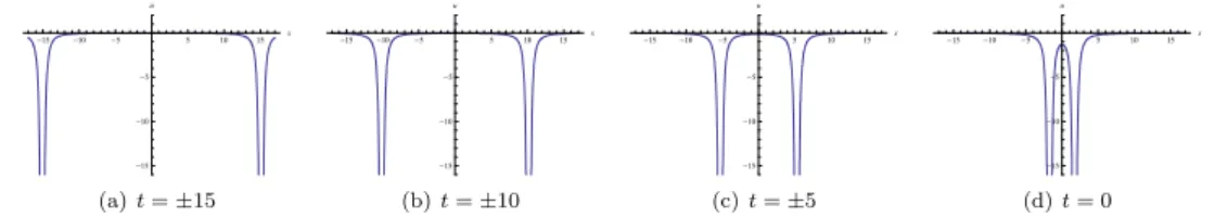
(3) 130 The fundamental rational rogue wave solution is obtained by the limit above solution. The limit can be taken for \sigma=-1 and we get. karrow 0. in the. f arrow\wedge t^{2}+x^{2}+3, u=4\frac{t^{2}-x^{2}+3}{(t^{2}+x^{2}+3)^{2} . This is a regular and time‐localized solution of Boussinesq I equation with \sigma=-1 . Fig. 2 shows time evolution of the above rogue wave solution which has time reversal symmetry. In the case of \sigma=+1 , we can not take the limit karrow 0 because of the condition k^{2}>\sigma,. (a). (b). t=\pm 20. (c). t=\pm 6. (d). t=\pm 2. Figure 2: (x, u) ‐plots of rational rogue wave solution for Boussinesq I equation with. t=0. \sigma=-1.. however we can start from the ansatz,. f=t^{2}+Ax^{2}+B , and determine constants. rational solution for. A. and. B. (9). from the bilinear eq. (4). Then we obtain a singular. \sigma=+1,. f=t^{2}-x^{2}+3, u=-4 \frac{t^{2}+x^{2}+3}{(t^{2}-x^{2}+3)^{2} , which describes repulsive interaction of a pair of singularities. Time evolution of this solution is shown in Fig. 3. For \sigma=0 , it is easy to check that there is no rational solution. (a). t=\pm 15. (b). (c). t=\pm 10. (d). t=\pm 5. t=0. Figure 3: (x, u) ‐plots of singular rational solution for Boussinesq I equation with \sigma=+1.. of the form of (9). By using the variable transformation (5), the Boussinesq II equation is transformed into. (D_{x}^{4}+aD_{x}^{2}+D_{t}^{2})f\cdot f=0 . Starting with the ansatz of perturbative form (6) and determining a blowing up breather solution exists for. solution for \sigma\leq 0 . For. \sigma>0 ,. \sigma>0. (10) \omega. and. A,. we find that. and there is no time‐localized breather. we have a singular breather solution (7) and (8) with. \omega=k\sqrt{\sigma-k^{2} , a=\sqrt{\frac{\sigma-4k^{2} {\sigma-k^{2} },.

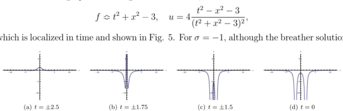
(4) 131 131 where k is a constant satisfying 4k^{2}<\sigma . This breather is a finite‐time blowing up solution but still localized in time, that is, singularities appear only in a finite interval around t=0. and the vanishing condition (3) is satisfied. This solution is shown in Fig. 4.. (a). t=\pm 2.5. (b). t=\pm 228. (c). (d). t=\pm 2.2. Figure 4: (x, u) ‐plots of finite‐time blowing up breather solution with with \sigma=+1.. k= \frac{1}{3}. t=0. for Boussinesq II equation. For \sigma=+1 , by taking the limit karrow 0 in the above blowing up breather, we get the finite‐time blowing up rational rogue wave solution,. f=t^{2}+x^{2}-3, u=4 \frac{t^{2}-x^{2}-3}{(t^{2}+x^{2}-3)^{2} , which is localized in time and shown in Fig. 5. For. (a). Figure 5:. t=\pm 2.5. (b). t=\pm 175. \sigma=-1 ,. (c). although the breather solution. (d). t=\pm 15. t=0. (x, u) ‐plots of finite‐time blowing up rational rogue wave solution for Boussinesq II equation. with \sigma=+1.. doesn’t exist, we have a rational solution. In fact substituting (9) into the bilinear form of Boussinesq II equation (10) and determining A and B , we get a singular solution,. f=t^{2}-x^{2}-3, u=-4 \frac{t^{2}+x^{2}-3}{(t^{2}-x^{2}-3)^{2} .. This solution is not localized in time and describes the annihilation and creation of a pair. of singularities (Fig. 6). There is no rational solution of the form of (9) for 3. \sigma=0.. Determinant structure of breather and rational solutions. For the Boussinesq I equation, the Akhmediev breathers can be superposed and the N‐ breather solution is given in terms of the Gram determinant,. f=1 \leq ij\leq Nd,et(\int_{-\infty}^{x}(e^{\xi_{\dot{x} +e^{\eta_{x} \cdot) (e^{\xi_{j}^{*} +e^{\eta_{j}^{*} )dx). =1\leqij\leqNd,et(\frac{e^{\xi_{}+\xi_{j}^{*} {p_{\dot{i}+p_{j}*+ \frac{e^{\xi_{x}+\eta_{j}^{*} {p_{i}+p_{j}+\frac{e^{\eta_{i}+\xi_{j}^{*} {p_{i}+p_{j}*+\frac{e^{\eta_{i}+\eta_{j}^{*} {p_{\dot{i}+p_{j}*). ,.

(5) 132. (a). (b). t=\pm 10. (c). t=\pm 5. (d). t=\pm 175. Figure 6: (x, u) ‐plots of singular rational solution for Boussinesq II equation with. t=0. \sigma=-1.. \xi_{j}=p_{j}x+i\sqrt{3}p_{\dot{j}}^{2}t+\xi_{j0}, \eta_{j}=p_{j}^{*}x+ i\sqrt{3}p_{j}^{*2}t+\eta_{j0}, where. p_{j},. \xi_{j0} and. \eta_{j0}. are arbitrary complex constants satisfying the reduction condition,. p_{j}^{2}+p_{j}p_{j}^{*}+p_{\dot{j} ^{*2}=- \frac{\sigma}{4}, N.. and {\rm Re} p_{j}>0 for j=1,2,. Here. *. denotes complex conjugate. Since f is the. determinant of positive definite Hermitian matrix,. u. in (5) gives regular solution. It. is straightforward to prove that the above f actually satisfies the bilinear Boussinesq I. equation (4) by using the Laplace expansion technique. The higher order rational solutions are also expressed in the determinant form,. f=|\begin{ar y}{l } m_{10} m_{1} \cdots m_{1,M-} m_{1,M+} m_{1,M+3} \cdots m_{1,2N- M1} m_{30} m_{31} \cdots m_{3,M-1} m_{3,M+1} m_{3,M+} \cdots m_{3,2N- M1} \vdots \vdots \vdots \vdots \vdots \vdots m_{2N-1,0} m_{2N-1,} \cdots m_{2N-1,M } m_{2N-1,M+} m_{2N-1,M+3} \cdots m_{2N-1,2N-M1} \end{ar y}|, m_{ij}=A_{i}B_{j} \frac{e^{(p+q)x+\sqrt{-3\epsilon}(p^{2}-q^{2})t} {p+q} p=q=\sqrt{-\frac{\sigma}{12}}. A_{i}= \sum_{k=0}^{i}\frac{a_{ik} {(i-k)!}(p\partial_{p})^{i-k} , (i=1,3, \cdots , 2N-1). ,. B_{j}=\{ begin{ar y}{l \sum_{l=0}^{j\frac{b_jl}{(j-l)!}(q\parti l_{q})^{j-l}, (j=M+1,M+3,\cdots ,2N-M1), \frac{1}\dot{j}!(q\parti l_{q})^{j}, (j=0,1 \cdots,M-1), \end{ar y}. a_{ik}= \sum_{r=0}^{k}\frac{3^{r+1}-1}{(r+2)!}a_{i+2,k-r} , (i=1,3, \cdots , 2N -3;0\leq k\leq i) b_{jl}= \sum_{s=0}^{l}\frac{3^{s+1}-1}{(s+2)!}b_{j+2,l-s} (j=M+1, M+3 2N-M-3;0\leq l\leq j) ,. ,. ,. where \epsilon is the sign \pm 1 in the left‐hand side of eq. (2) and 0\leq M\leq N . Here a_{2N-1,k} (0\leq k\leq 2N-1) and b_{2N-M-1,l}(0\leq l\leq 2N-M-1) are arbitrary constants, however they are not independent and we can take a_{2N-1,0}=1, a_{2N-1,2k}=0(1\leq k\leq N-1) ,.

(6) 133 b_{2N-M-1,0}=1, b_{2N-M-1,2l}=0(1 \leq l\leq\frac{2N-M-1}{2}) without loss of generality. The coefficients a_{ik}(1\leq i\leq 2N-3) and b_{jl}(M+1\leq j\leq 2N-M-3) are recursively defined in the above way. The elements m_{ij} of determinant are given by the parameter derivatives. We can prove that the above f actually satisfies the bilinear form of Boussinesq equation. in the same way with the case of NLS equation [5].. It should be pointed out that the above f is written in the form of two component determinant, that is, we have N\cross M matrix (m_{2i-1,j-1})_{1\leq i\leq N,1\leq j\leq M} on left, and N\cross (N-M) matrix (m_{2i-1,2j-M-1})_{1\leq i\leq N,M+1\leq j\leq N} on right in the determinant. For soliton equations of complex variables such as NLS equation, the rational solutions are expressed by the single component Gram determinant which corresponds to the case of M=0 . This is because we need M=0 to satisfy the complex conjugate condition. For real variable equations such as Boussinesq equation, the determinant solutions are not restricted by the conjugate condition and we have a free parameter M . Thus a wider class of rational solutions is obtained when the reality condition of f is satisfied. However it is still unclear whether those solutions are regular and whether they are localized in time.. 4. Other equations. The bilinear method can be applied to nonintegrable equations also. In general the bilinear equation,. P(D)f\cdot f=0, where P(D) is a polynomial of D_{x}, D_{y}, D_{t} , . . ., admits at least 2‐soliton solution and 1‐breather solution of the form,. f=1+e^{\xi}+e^{\xi^{*}}+Ae^{\xi+\xi^{*}} \xi=px+qy+\omega t+ Thus it might be possible to find regular and time‐localized breather solutions among the above f . One simple example is the bilinear equation,. (D_{x}^{4}+\sigma D_{y}^{2}-D_{t}^{2})f\cdot f=0, which is transformed to. u_{tt}=u_{xxxx}+3(u^{2})_{xx}+\sigma u_{yy}, through the variable transformation (5). This equation admits the breather solution,. far ow\wedge\sqrt{\frac{4k^{4}-\sigma l^{2} {k^{4}-\sigma l^{2} }\cosh(\sqrt{k^ {4}-\sigma l^{2} t)-\cos(kx+ly) where k and solution,. l. are constants satisfying k^{4}>\sigma l^{2} , and if. \sigma=-1 ,. we have the rational. farrow-t^{2}+(kx+y)^{2}+3k^{4}.. Another example of bilinear equation,. (D_{x}^{4}+D_{x}^{2}D_{y}^{2}-D_{t}^{2})f\cdot f=0, is transformed to. u_{tt}=u_{xxxx}+3(u^{2})_{xx}+u_{xxyy}+(2v_{x}^{2}+uv_{y})_{xx}, u_{y}=v_{xx},. ,.

(7) 134 by the variable transformations (5) and v=(2\log f)_{y} . This equation has the time‐ localized breather solution,. farrow\wedge 2\cosh(k\sqrt{k^{2}+l^{2}}t)-\cos(kx+ly). ,. and we also find another breather type solution,. f-2\cosh(\sqrt{2}ky)\cosh(k^{2}t)-\sinh(\sqrt{2}ky)\cos(kx). ,. by straightforward calculation. The bilinear formalism provides a simple and useful way to construct these kinds of solutions and the equations admitting such solutions simulta‐ neously.. 5. Concluding remarks. According to the signs of coefficients, there are various types of solutions of the Boussi‐. nesq eq. (2), such as the Akhmediev breather, rational rogue wave, finite‐time blowing up breather, finite‐time blowing up rational rogue wave and solutions of interacting singular‐ ities. Only some cases of the equations and solutions are relevant for the nonlinear water waves, but the Boussinesq equations may appear in some other contexts of physics. It might be interesting to study interpretations of those solutions in various physical systems. The multi Akhmediev breathers and higher order rational solutions are presented in the determinant form. The multi Akhmediev breather solutions are regular and describe time‐localized excitation of waves. Investigating properties of the higher order rational solutions including regularity and time‐localization may be a future work. References. [1] N. Akhmediev, A. Ankiewicz and M. Taki, Phys. Lett. A 373 (2009) 675. [2] N. Akhmediev, J. M. Soto‐Crespo and A. Ankiewicz, Phys. Lett. A 373 (2009) 2137. [3] D. H. Peregrine, J. Austral. Math. Soc. Ser. B 25 (1983) 16. [4] P. Dubard, P. Gaillard, C. Klein and V. B. Matveev, Eur. Phys. J. Special Topics 185 (2010) 247.. [5] Y. Ohta and J. Yang, Proc. R. Soc. A 468 (2012) 1716. [6] P. A. Clarkson and E. Dowie, Trans. Math. Appl. 1 (2017) 1. [7] A. Ankiewicz, A. P. Bassom, P. A. Clarkson and E. Dowie, Stud. Appl. Math. 139 (2017) 104.. [8] Z. Dai, C. Wang and J. Liu, Pramana‐J. Phys. 83 (2014) 473..

(8)