Problems on Low-dimensional Topology, 2017 (Intelligence of Low-dimensional Topology)

全文

(1)121. 数理解析研究所講究録第2052巻 2017年 121-138. Problems. on. Edited. Low‐dimensional by. Tomotada Ohtsuki and. Topology,. 2017. Tetsuya Ito2. a list of open problems on low‐dimensional topology with expositions of history, background, significance, or importance. This list was made by editing manuscripts written by contributors of open problems to the problem session of the conference Intelligence of Low‐dimensional Topology held at Research Institute for Mathematical Sciences, Kyoto University in May 24‐26, 2017.. This is. their. Contents 1. The AJ. 2. Loop finite type invariants of null‐homologous homology 3‐spheres. 3 4. conjecture. The double. for cable knots. covering. Presentations of. 2. knots in rational 3. method for twisted knots. (immersed). surface‐knots. 5. marked. by. graph. dia‐ 6. grams 5. Knotted 2‐foams and. 6. 3‐dimensional braids. 7. Volume. 8. Gauge theory. lResearch. conjecture on. quandle homology. 9 10. for 3‐manifolds. 10. 4‐manifolds with \mathb {Z} ‐actions. Institute for Mathematical. 14. Sciences, Kyoto University, Saky $\sigma$-\mathrm{k}\mathrm{u} Kyoto, 606‐8502, ,. JAPAN. Email: [email protected]‐u.ac.jp The first editor is partially supported by JSPS KAKENHI Grant Numbers 16\mathrm{H}02145 and 16\mathrm{K}13754.. 2Department. of. Mathematics, Graduate School. of. Science, Osaka University. 1‐1. Machikaneyama Toyonaka,. Osaka 560‐0043, JAPAN Email: [email protected]‐u.ac.jp The second editor is. partially supported by JSPS KAKENHI Grant. 1. Numbers 15\mathrm{K}17540 and 16\mathrm{H}02145..

(2) 122. The AJ. 1. (Anh. T. Th. for cable knots. conjecture. an). conjecture relates the \mathrm{A} ‐polynomial and the colored Jones polynomial The \mathrm{A} ‐polynomial A_{K}(M, L) of a knot K \subset S^{3} was introduced by Cooper et al. [11]; it describes the character variety of the knot complement as viewed from the boundary torus. For every knot K Garoufalidis and Le [16] proved that the colored Jones polynomial J_{K}(n) \in \mathbb{Z}[t^{\pm 1}] with the color n standing for the The AJ. of. a. knot in S^{3}. .. ,. ,. sl_{2}(\mathbb{C}) ‐module of dimension n satisfy linear recurrence relations. The recurrence polynomial $\alpha$_{K}(t, M, L) of K is the minimal linear recurrence relation for J_{K}(n) Motivated by the work of Frohman, Gelca and LoFaro [12] on the non‐ commutative \mathrm{A} ‐ideal, Garoufalidis [14] proposed the AJ conjecture which states that $\alpha$_{K} |_{t=-1} is equal to A_{K}(M, L) up to multiplication by a polynomial depending on irreducible. ,. .. M. only. Suppose K is knot K^{(r,s)} of K. relatively prime integers. The (r, s) ‐cable boundary of K A cabling formula for the \mathrm{A} ‐polynomial has recently been given by Ni and Zhang [42]. For a pair of relatively prime integers (r, s) with s\geq 2 define F_{(r,s)}(M, L) \in \mathbb{Z}[M, L] by a. knot and r,. is the. s are. (r, s) ‐curve. two. on. the torus. .. ,. F_{(r,s)}(M, L)= Then. \left\{ begin{ar y}{l M^{2r}L+1&\mathrm{i}\mathrm{f}s=2,\ M^{2rs}L^{2}-1&\mathrm{i}\mathrm{f}s>2. \end{ar y}\right.. A_{K(r,\mathrm{s})}(M, L)=(L-1)F_{(r,s)}(M, L){\rm Res}_{\ell}(\displaystyle \frac{A_{K}(M^{s},\ell)}{\ell-1}, \ell^{s}-L). where {\rm Res}_{\ell} denotes the polynomial resultant eliminating the variable \ell. On the other hand, a cabling formula for the colored Jones polynomial. by. Morton. was. given. [36]:. J_{K}(r,s)(n)=t^{-rs(n^{2}-1)}\displaystyle \sum_{j=-(n-1)/2}^{(n-1)/2}t^{4rj(sj+1)}J_{K}(2sj+1). We define 2 linear operators. L,. M. acting. on. one can. relate the colored Jones. polynomials. of. (2). .. f : \mathbb{Z}\rightar ow \mathbb{C}[t^{\pm 1}] by. discrete functions. (Lf)(n)=f(n+1) , (Mf)(n)=t^{2n}f(n) Using (2),. (1). ,. .. K^{(r,s)} and. K. as. follows:. t^{2rs}M^{rs}(L^{2}-t^{-4rs}M^{-2rs})J_{K(r,s)}(n). = t^{2r(n+1)}J_{K}(s(n+1)+1)-t^{-2r(n+1)}J_{K}(s(n+1)-1) Moreover,. in. case. of. (r, 2) ‐cable. knots. one. has. M^{r}(L+t^{-2r}M^{-2r})J_{K}(r,2)(n)=J_{K}(2n+1) These. equalities. K and its cable. should. K^{(r,s)}. .. imply. a. .. relationship. It is ideal is to have. between the a. .. recurrence. similar formula to. (1). polynomials such. $\alpha$_{K(r,s)}(-1, M, L)=(L-1)F_{(r,s)}(M, L){\rm Res}_{\ell}(\displaystyle \frac{$\alpha$_{K}(-1,M^{s},\ell)}{\ell-1}, \ell^{s}-L) 2. of. as. (3).

(3) 123. up to. multiplication by. Problem 1.1. (A.. T.. a. polynomial depending. Tran).. Prove. equality (3) for. If K satisfies the AJ conjecture and (3) holds K^{(r,s)} satisfies the AJ conjecture.. 2. M. on. finite type invariants of rational homology 3‐spheres. Loop. only.. all cable knots. true for. K^{(r,s)}.. cable knot. a. K^{(r,s)} then ,. knots in. null‐homologous. (Delphine Moussard) loop finite type invariants of null‐homologous knots in rational homology 3‐ spheres, there are two candidates to be universal loop finite type invariants, namely the Kricker rational lift of the Kontsevich integral [27, 15] and the Lescop invariant constructed by means of equivariant intersections in configuration spaces [31]. Le‐ scop conjectured in [32] that these two invariants are equivalent for null‐homologous knots in rational homology 3‐spheres with a given Blanchfield pairing and a given cardinality for the first homology group of the manifold; we recall that the Blanch‐ field pairing is the equivariant linking pairing on the universal cyclic cover of the knot complement. By equivalent, we mean that one invariant distinguishes two knots if and only if the other invariant distinguishes them. é first recall some definitions. Let (M, K) be a \mathbb{Q}SK‐pair, i.e a pair of a rational ) logy 3 ‐sphere M and a null‐homologous knot K in M Let A\subset M\backslash K be a rational homology handlebody ( \mathb {Q} ‐handlebody). Assume A is null in M\backslash K, i.e. the map incl* : H_{1}(A, \mathbb{Q}) \rightarrow H_{1}(M\backslash K, \mathbb{Q}) has a trivial image. Let B be another \mathb {Q} ‐handlebody with the same genus. Fix a homeomorphism h : \partial A \rightarrow \partial B The \mathb {Q}\mathrm{S}\mathrm{K} ‐pair obtained from (M, K) by the null Lagrangian‐preserving surgery, or null LP‐surgery, (\displaystyle \frac{B}{A}) is: For. .. .. .. (M, K)(\displaystyle \frac{B}{A})=( M\backslash Int(A) \bigcup_{h}B, K). .. \mathcal{F}_{0} be the rational vector space spanned by all QSK‐pairs up to orientation‐ preserving homeomorphism. Let \mathcal{F}_{n} be the vector subspace of \mathcal{F}_{0} spanned by the Let. [(M, K);(\displaystyle \frac{B_{1} {A_{1} ), . . , (\frac{B_{n} {A_{n} )]=\sum_{I\subset\{1,. n\} .,(-1)^{|I}(M, K)( \frac{B_{i} {A_{i} )_{i\in I}) for all. \mathb {Q}\mathrm{S}\mathrm{K} ‐pairs (M, K). all families of. A_{n} null disjoint \mathb {Q}‐handlebodies A_{1} ‐ handlebodies with a fix identification B_{1} B_{n} \ m a t h b { Q } M\backslash K \partial B_{i}\cong\partial A_{i} Since \mathcal{F}_{n+1} \subset \mathcal{F}_{n} this defines a filtration of \mathcal{F}_{0}. .. Definition. QSK‐pairs. ,. ,. and all families of. in. ,. .. .. .. .. .. .. ,. ,. ,. \mathrm{A}. \mathb {Q} ‐linear. if. $\lambda$(\mathcal{F}_{n+1})=0.. map $\lambda$. :. \mathcal{F}_{0}\rightar ow \mathbb{Q}. is. 3. a. loop finite type. invariant. of degree. n. of.

(4) 124. homeomorphism classes of QSK‐pairs up to null LP‐surgeries are characterized isomorphism classes of their Blanchfield pairings [37]. Therefore, the Blanch‐ field pairing dominates degree 0 invariants. The degree 1 invariants are given by the cardinality of the first homology group of the manifold. The. by. the. Question the Lescop. 2.1. (D. Moussard).. invariant universal. Are the Kricker. loop finite type. lift of. the Kontsevich. invariants. of \mathbb{Q}SK‐pairs. integral and degree. up to. 0 and 1 invariants ?. Since these two invariants satisfy the same splitting formulas with respect to null LP‐surgeries [32, 38], the answer should be the same for both invariants. Note that Question 2.1 implies Lescops conjecture. The answer is known to be positive when the Blanchfield pairing is trivial [39].. Since the Blanchfield pairing dominates degree 0 invariants, the space \mathcal{F}_{0} is the sum over all isomorphism classes of Blanchfield pairings \mathfrak{B} of spaces \mathcal{F}_{0}(\mathfrak{B}) and the filtration (\mathcal{F}_{n})_{n\in \mathbb{N} splits accordingly into filtrations (\mathcal{F}_{n}(\mathfrak{B}) _{n\in \mathbb{N} of each. direct. \mathcal{F}_{0}(\mathfrak{B}). ,. .. Denote. \mathcal{G}_{n}(\mathfrak{B}). =. \mathcal{F}_{n}(\mathfrak{B})/\mathcal{F}_{n+1}(\mathfrak{B}). given Blanchfield pairing \mathfrak{B} we have a the connected sum of QSK‐pairs with pairing \mathfrak{B}. ,. Question. 2.2. (D. Moussard).. 1\leq 2k<3n is the ,. The bound. on. map. a. a. C_{n}. fixed. :. quotients of the filtration.. \mathcal{G}_{n}(\mathfrak{B}^{\oplus k})\rightar ow \mathcal{G}_{n}(\mathfrak{B}^{\oplus k+1}). QSK‐pair (M_{0}, K_{0}). Blanchfield pairing. C_{n}:\mathcal{G}_{n}(\mathfrak{B}^{\oplus k})\rightar ow \mathcal{G}_{n}(\mathfrak{B}^{\oplus k+1}). the value of k. [39] when N \geq Kricker lift of the Kontsevich described in. type invariants of degree. Given. map. the. comes. \displayst le\frac{3}2n. for. non‐zero. and at most 2n. .. a. In. established: Fact. For. all. n. a. given Blanchfield pairing, Question. 2.1 is. induced. a. by. with Blanchfield. integers k,. with. n. injective /?. from the fact that. In. particular, integral and the Lescop .. \mathfrak{B} and. For. \mathcal{G}_{n}(\mathfrak{B}^{\oplus N}). combinatorially pairing \mathfrak{B}^{\oplus 3n} the dominate loop finite is. Blanchfield invariant. [39],. the. ,. following. equivalent. to. fact is also. Question. 2.2 for. and k.. About. Question 2.2, we shall mention a result of existence and uniqueness of the decomposition of a \mathb {Q}\mathrm{S}\mathrm{K} ‐pair as the connected sum of irreducible \mathb {Q}\mathrm{S}\mathrm{K} ‐pairs [35]. Unfortunately, such a decomposition is not preserved by null LP‐surgeries.. loop‐degree of a Jacobi diagram on S^{1} is defined to be given by the number of trivalent vertices minus the number of univalent vertices of the uni‐trivalent graph of the Jacobi diagram. The filtration of the space of Jacobi diagrams on S^{1} given by loop‐degrees is related to the filtration of loop finite type invariants through the rational lift of the Kontsevich integral. The theory of this filtration is developed in [17] (noting that this notion also appears in [26] and the September 1999 version of [28]); see also [44, Section 2.9]. Remark. (T. Ohtsuki).. The. half of the number. 4.

(5) 125. The double. 3. method for twisted knots. covering. (Naoko Kamada)3 by L. H. Kauffman [24] as a generalization diagrams and link diagrams in closed oriented surfaces. A virtual link diagram is a link diagram possibly with virtual crossings, and a virtual link is an equivalence class of such diagrams by some Reidemeister type moves. Virtual links correspond to stable equivalence classes of links in oriented 3‐ Virtual knot. of knot. theory. theory. based. manifolds which. are. on. was. introduced. Gauss chord. line bundles. over. closed oriented surfaces. ([6,. Twisted. 22. Bourgoin [1]. diagram possibly with virtual crossings and bars on arcs, and a twisted link is an equivalence class of such diagrams by some Reidemeister type moves. Twisted links correspond to stable equivalence classes of knot. introduced. theory theory. A twisted was. link. by diagram. M. O. is. a. links in oriented 3‐manifolds which. ([1,. closed surfaces. an. extension of virtual knot. link. are. line bundles. over. (possibly non‐orientable). 6. An abstract link. |D|. It is. diagram. is. a. link. diagram. |D|. deformation retract of $\Sigma$ , where. D. on a. a. is the. compact surface $\Sigma$ such that. immersed loops in $\Sigma$ by forgetting over/under information from D In [22] and [1], an equivalence relation An abstract link is an equivalence classes of on abstract link diagrams is defined. abstract link diagrams by the equivalence relation. There is a bijection from the set is. underlying. .. of virtual links and the set of abstract links a. bijection. on. orientable surfaces. [22],. from the set of twisted links and the set of abstract links. An abstract link. Definition.. diagram. D. on. $\Sigma$ is normal. or. on. and there is. [1].. surfaces. checkerboard colorable if. $\Sigma$\backslash |D|\cup(bars) is checkerboard colorable. (Namely, we can assign elements of \mathbb{Z}/2\mathbb{Z} regions of $\Sigma$\backslash |D|\cup(bars) such that two regions sharing an arc (or a bar) are assigned distinct values.) A virtual link diagram or a twisted link diagram is normal if the corresponding abstract link diagram (in the sense of [22]) is normal. A virtual. to. link. or a. twisted link is normal if there is. (or twisted). link. Problem 3.1. a. representative which. is. a. normal virtual. diagram.. (N. Kamada).. Construct invariants. of normal. virtual links.. signature is defined for normal virtual links [20]. conference, a method of obtaining a virtual link diagram from a twisted link diagram, called the double covering method ([23]). Using this method, we obtain a method of converting any virtual link diagram with a cut system to a normal virtual link diagram. (A cut system of a virtual link diagram D is a finite number of points C on arcs of D such that when we put bars at the points of C we obtain a normal twisted link diagram. Then the double covering of such a normal twisted link diagram is a normal virtual link diagram. This is the method of the con‐ version. The resulting normal virtual link diagram depends on the cut system C for D but its \mathrm{K} ‐equivalence class is uniquely determined from D Here \mathrm{K} ‐equivalence For. example,. the. In the talk at the. ,. .. ,. 3Supported by. JSPS KAKENHI Grant Number 15\mathrm{K}04879.. Graduate School of Natural Aichi 467‐8501. Sciences, Nagoya City University,. Japan. 5. 1. Yamanohata, Mizuho‐cho,. Mizuho>\mathrm{k}\mathrm{u} ,. Nagoya,.

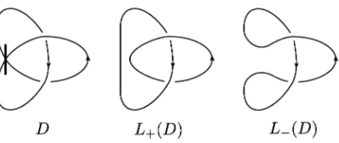
(6) 126. is the. equivalence. relation. an. (N. Kamada).. Problem 3.2. normal virtual link.. find. on. for virtual links and. moves. Using. virtual link additional. diagrams. Find another method. the. method,. modulo the Reidemeister type. flype.). called Kauffmans. move. construct. of converting. a new. virtual link to. a. of virtual. invariant. links. a. or. application.. an. An abstract link. diagram D on oriented $\Sigma$ is almost classical or region namely, we can assign elements of \mathb {Z} to regions of $\Sigma$\backslash |D| such that if the right side is assigned i with respect to the orientation of the A virtual link diagram is almost classical if arc then the left side is assigned i+1 the corresponding abstract link diagram is almost classical. A virtual link is almost classical if there is a representative which is an almost classical virtual link diagram.. Definition.. \mathb {Z} ‐colorable if. $\Sigma$\backslash |D|. is \mathb {Z} ‐colorable,. .. By. the. projection \mathbb{Z}\rightar ow \mathbb{Z}/2\mathbb{Z}. Problem 3.3. (N. Kamada).. Problem 3.4. (N. Kamada).. classical virtual link. or. find. an. Using. almost virtual link is. Construct invariants Find the. a. method. method,. almost classical virtual links.. of. of converting. construct. normal virtual link.. a. a. a new. virtual link to. invariant. of. an. almost. virtual links. application.. Presentations of. 4. an. ,. (immersed). surface‐knots. by. marked. graph. diagrams (Jieon Kim)4 An immersed surface‐knot is. 4‐space \mathbb{R}^{4}. A marked graph diagram. a. generically. immersed closed and connected surface. in the. is. a. vertex with. marked. a. a. diagram. marker looks like. graph diagram. vertex looks like. For. a. is. \times\cdot. in which every. \ovalbox{\t smal REJ CT}\mathrm{o}\mathrm{r}\ovalbox{\t smal REJ CT}.. of. edge. a. 4‐valent. link. diagrams. \wedge^{\mathrm{a}\mathrm{n}\mathrm{d}\ve ) (. ,. obtained from D. respectively. A. marked. each of whose vertices. An oriented marked has. an. given (oriented) marked graph diagram. (oriented). graph. graph diagram. is. a. orientation such that each marked. D , let. L_{+}(D). by replacing each. graph diagram. and. L_{-}(D). be classical. marked vertex. \times. with. D is said to be H‐admissible. L_{+}(D) and L_{-}(D) are \mathrm{H} ‐trivial link diagrams, where an \mathrm{H} ‐trivial split union of trivial knots and Hopf links. See Fig. 1. An unlinking crossing point c of a classical link diagram L is a crossing of L such that L is transformed into a diagram of an unknotted link by switching over arc and if both resolutions link is. a. under. arc. 4(Osaka. of. c.. city University /JSPS). 6.

(7) 127. L_{-}(D). L_{+}(D). D. Figure. 1: \mathrm{H} ‐admissible marked. graph diagram. Definition. A crossing point p (in a marked graph diagram D ) is an upper singular point if p is an unlinking crossing point in the resolution L_{+}(D) and a lower singular point if p is an unlinking crossing point in the resolution L_{-}(D) respectively. ,. ,. Remark. The. ponents l^{+}. (a) of $\Gamma$_{9} and $\Gamma$_{9}' in Fig. 4 need the conditions that the com‐ the resolution L_{+}(D) ) and l^{-} (in the resolution L_{-}(D) ) are trivial,. moves. (in. respectively. The moves (b) of $\Gamma$_{9} and $\Gamma$_{9}' need the conditions singular point and a lower singular point, respectively. It is known that two marked. and. The. if. only they generalized. are. related. Yoshikawa. by. that p. graph diagrams present equivalent. the Yoshikawa. moves. for marked. graph. moves. ,. .. .. ,. ,. Definition. of. moves. in. A set S of. S\backslash \{x\}. .. .. .. surface‐links if. ,. moves are. independent if x. Lemma. Let \mathcal{L} and \mathcal{L}' be immersed. diagrams, respectively.. (J. Kim).. are. surface‐links. Problem 4.3. graph diagrams equivalent.. (J. Kim).. are. generated by. shown in. finite sequences. Create. Kim, S.. related. Y. Lee. [21]).. Is the set. of. and D and D' their marked. by. a. finite sequence of. graph generalized. equivalent.. Find the set S. such that the marked. J.. surface‐links,. If D and D'. Yoshikawa moves, then \mathcal{L} and \mathcal{L}'. are. is not. as. for every x\in S.. Question 4.1 (S. Kamada, A. Kawauchi, generalized Yoshikawa moves independent?. Problem 4.2. upper. of type I and type II (see [49]). diagrams are the deformations. $\Gamma$_{5} (Type I), $\Gamma$_{6} $\Gamma$_{8} (Type II), and $\Gamma$_{9}, $\Gamma$_{9}', $\Gamma$_{10} (Type III) and Fig. 2, Fig. 3, Fig. 4, respectively. $\Gamma$_{1}. .. are an. are. of. local. related. by. S. if. of. marked. and. only if. graph diagrams their immersed. of H‐admissible marked graph diagrams rep‐ equivalence of S in the previous Problem resenting surface‐links with ch‐index 10 or less, where the ch‐index of a marked graph diagram is the sum of the number of crossings and that of vertices. immersed. a. table. moves. under the. 7.

(8) 128. Figure. 2: Moves of. Type. I. Figure. 3: Moves of. Type. II. 8.

(9) 129. Figure. Knotted 2‐foams and. 5. (J.. Scott. 4: Moves of. Type. III. quandle homology. Carter). Let. $\Delta$^{n+1}=\displaystyle \{\vec{x}= (x_{0}, x_{1}, \cdot \cdot \cdot , x_{n+1})\in \mathbb{R}^{n+2} | \sum x_{i}=1 \& 0\displaystyle \leq x_{i}\} denote the standard. (\displaystyle\frac{1}{2},\frac{1}{2}). Take. .. to the. simplex.. The space Y^{n} \subset $\Delta$^{n+1} is defined Embed a copy,. $\Delta$_{j}^{n}=\{\vec{x}\in$\Delta$^{n+1}|x_{j}=0\}. barycenter. b=\displaystyle \frac{1}{n+2}(1,1, \ldots, 1). .. of $\Delta$^{n+1}. .. We put. Y^{n}=C(\displaystyle \bigcup_{j=1}^{n+2}Y_{j}^{n-1}). Y_{j}^{n-1}\subset$\Delta$_{j}^{n}. as .. follows: Y^{0}. Cone. \displaystyle \bigcup_{j=1}^{n+2}Y_{j}^{n-1}. .. An. n ‐foam is a compact topological space X for which each point x \in neighborhood N(x) that is homeomorphic to a neighborhood of a point in. Y_{0}. Y_{1}. =. X has. a. Y^{n}.. Y_{2}. particular, a 2‐foam is a compact topological space such that any point has a neighborhood that is homeomorphic to a neighborhood of a point in Y_{2} A knotted 2‐foam is an embedded 2‐foam in a 4‐dimensional space. A knotted 2‐foam is a 2‐dimensional generalization of a spatial trivalent graph. See [4, 3] for details. In. .. Carter, see [3, Problem 3.5]). Construct interesting examples 2‐foams by using movie techniques.. Problem 5.1. of. knotted. This In. problem a. (J.. S.. is related to the next. group, let. problem. we have,. a\triangleleft b=b^{-1}ab Then .. 9.

(10) 130. YY. (ab)c=a(bc). YI. (ab)\triangleleft c=(a\triangleleft c)(b\triangleleft c). IY. (a\triangleleft b)\triangleleft c=a\triangleleft(bc). III. (a\triangleleft b)\triangleleft c=(a\triangleleft c)\triangleleft(b\triangleleft c). crossings of 2‐foams are geometric representations of chains in the homology algebraic structure encoded by these four identities. There is a homology theory that encompasses both group and quandle homology. (See for example, this volume or my talk at RIMS). Local. that is associated to the. (J. S. Carter). Develop for foam homology.. Problem 5.2 ogy classes. 6. (J.. methods. of computing homology. and cohomol‐. 3‐dimensional braids. Carter). Scott. [5]. Carter and Kamada. beddings. or. branched. along. Let D^{2} be. a. a. a method for constructing simple braided em‐ 5‐space of the 2‐fold and 3‐fold branched covers of S^{3}. described. immersions in. given knot. link.. or. : D^{2}\times S^{3}\rightarrow S^{3} the second factor projection. S^{3} of degree d is a 3‐manifold M such that the S^{3} is a simple branched covering map of degree d. 2‐disk. We denote. A 3‐dimensional braid in D^{2} restriction map branched along. pr_{2}|_{M} a. :. M. link in S^{3}. map whose. \rightarrow. \times. by pr_{2}. Here, a simple branched covering map is a branched monodromy takes each meridian of the link of the branch set .. covering a transposition. See [5] for details of 3‐dimensional braids. We consider 3‐dimensional braids of degree 2 or 3.. to. Question. (1) (2). When. 6.1 are. (J.. S.. Carter).. these knotted?. particular, are the embeddings that are constructed via the Seifert algorithm for given diagram knotted.? (3) What are the relationships among the immersions of the 2‐fold branched covers that are parametrized by the bracket smoothing cube? Explicitly modify the Seifert algorithm to construct (possibly non‐orientable) surfaces using any combination of A and B smoothings. Can the immersions in 5‐space be isotopic Í? In. a. 7. Volume. conjecture. for 3‐manifolds. (Qingtao Chen) Yang [10],. proposed the Volume Conjecture for Reshetikhin‐ Turaev and Turaev‐Viro invariants at roots of unity q(2) where q(s) e^{s $\pi$\sqrt{-1}/r}. The example of Turaev‐Viro invariant of non‐orientable 3‐manifold N_{2_{1}} (Callahan‐ Hildebrand‐Weeks census [2]) vanishes at roots of unity q(s) where r and s are In my paper with T.. we. =. ,. ,. 10.

(11) 131. both odd numbers and. invariant).. Turaev‐Viro. also goes exponentially r is an even number.. (r, s)=1 (required by. a. when. s. condition from the definition of the. Numerical evidence shows that it is. large. as. r\rightarrow\infty ,. Thus it is natural to propose the. following. is. nonzero. at. q(s). and. odd number other than 1 but. an. Volume. Conjecture,. Conjecture 7.1 (Q. Chen). Let M be an (orientable or non‐orientable) hyperbolic 3‐manifold with cusps or totally geodesic boundary. For a fixed odd number s other than 1 and such integer r that condition (*) TV_{r}(M, q(s)) \neq 0 is satisfied, then we have. \displaystyle \lim_{r\rightar ow\infty} \underline{s $\pi$}_{\log}|TV_{r}(M, q(s) | = \mathrm{V}\mathrm{o}\mathrm{l}(M). r. If. Remark.. boundary,. .. r. (r,s)=1. satisfies (*). TV_{r}(M, q(s))\neq 0 could. we. for all any even integer r and any 3‐manifold M with condition r satisfies (*) to r is even. change. When M has cusps, as in [10], we consider ideal tetrahedral decomposition of M , and consider Turaev‐Viro invariant of this tetrahedral decomposition. Remark.. totally geodesic boundary, we consider the singular 3‐manifold by collapsing each boundary component, and consider Turaev‐ of a triangulation of this singular 3‐manifold.. When M has. obtained from M Viro invariant. Similar. to the Reshetikhin‐Turaev invariants also.. phenomenon happens. Reshetikhin‐Turaev invariants of closed 3‐manifold M obtained from. along. a. K, RT_{r}(M, q(s)) vanishes. knot. at roots of. ,. (r, s). both odd numbers and. =. (see [25]. 1. shows that Reshetikhin‐Turaev of certain and also goes exponentially but r is an even number.. large. and. examples. as r\rightarrow\infty ,. Thus it is natural to propose the. see. when. following. s. a. unity q(s) where ,. [9]).. also. we. is. Volume. tested. an. The. 4k+2 ‐surgery r. and. s. are. Numerical evidence are nonzero. at. q(s). odd number other than 1. Conjecture,. Conjecture 7.2 (Q. Chen). Let M be a closed hyperbolic hyperbolic 3‐manifold. For a fixed odd number s other than 1 and such integer r that condition (**) RT_{r}(M, q(s))\neq 0 is satisfied, then we have. rs. with. *)(r\displaystyle\vec{s)},=1\lim_{r\infty}\frac{2s$\pi$}{r}\log(RT_{r}(M,q(s). =. \mathrm{V}\mathrm{o}\mathrm{l}(M)+\sqrt{-1} CS (M). (mod \sqrt{-1}$\pi$^{2}\mathbb{Z} ),. atisfies ( a. suitable choice. Remark.. If. manifold M , Habiro. invariants). of. a. branch. RT_{r}(M, q(s)) \neq 0 we. could. change. [18, 19] proved of. a. knot K. of. the. \mathrm{l}\mathrm{o}\mathrm{g}.. for all any condition. integer. even r. satisfies. be. expanded. in the. 11. (**). . and any 3‐manifold closed to r is even. polynomial (reduced colored SU(2) following form, called the cyclotomic. that the colored Jones. can. \mathrm{r}.

(12) 132. expansion,. J_{0}(K) = 1, J_{1}(K) = 1+\{1\}\{3\}H_{1}(K) J_{2}(K) = 1+\{2\}\{4\}H_{1}(K)+\{1\}\{2\}\{4\}\{5\}H_{2}(K) ,. ,. :. J_{N}(K) for. some. 1 +. =. H_{i}(K) \in \mathbb{Z}[q]. polynomial. \{N\}\{N+2\}H_{1}(K) + + \{1\}\cdots\{N\}\{N+2\}\cdots\{2N+1\}H_{N}(K). where. ,. .. \{n\}=q^{n}-q^{-n}. associated with the N‐th. .. J_{N}(K). and. symmetric. .. tensor. ,. denotes the colored Jones. product of. the fundamental. representation of \mathcal{B}1_{2} ( i.e. , the (N+1) ‐dimensional irreducible representation of \mathcal{B}l_{2} ). Careful readers who are familiar with Volume Conjecture may find that root of. unity employed in Volume Conjecture proposed by Kashaev‐Murakami‐Murakami is exactly q=e^{\frac{ $\pi$}{N+1}} which is a solution of gap equation \{N+1\}=0 in cyclotomic expansion. ,. The colored. SU(n). invariant. variant associated with the N‐th resentation of. J_{N}^{SU(n)}(K). symmetric. of. a. knot K is the quantum SU(n) in‐ product of the fundamental rep‐. tensor. \mathfrak{s}$\iota$_{n}.. Conjecture 7.3 (Chen‐Liu‐Zhu [9]). be expanded in the following form,. J_{0}^{SU(n)}(K) J_{1}^{SU(n)}(K) J_{2}^{SU(n)}(K). =. =. =. The colored. SU(n). invariants. of a. knot K. can. 1,. 1+\{1\}\{n+1\}H_{1}^{SU(n)}(K) 1+\{2\}\{n+2\}H_{1}^{SU(n)}(K)+\{1\}\{2\}\{4\}\{5\}H_{2}^{SU(n)}(K) ,. ,. :. J_{N}^{SU(n)}(K) for. some. =. 1 +. H_{i}^{SU(n)}(K). \{N\}\{N+n\}H_{1}^{SU(n)}(K) + + \{1\}\cdots\{N\}\{N+n\}\cdots\{2N+n-1\}H_{N}^{SU(n)}(K) .. .. .. ,. \in \mathbb{Z}[q].. Conjecture 7.4 (Chen‐Liu‐Zhu [9]). Volume Conjecture holds for the colored SU(n) invariants of a knot K at roots of unity q e^{\frac{ $\pi$}{N+a}} (with a wider choices), where =. a=1,. n-1.. proved the conjecture in the case of the figure‐eight knot. We note that these 0 in the above cyclotomic corresponds to the gap equation \{N+a\} expansion.. We. roots. =. [7] applied this philosophy to the (reduced) superpolynomial of HOMFLY‐ homology and Kauffman homology and thus obtained both cyclotomic expansion. Chen PT. 12.

(13) 133. Conjectures (proved. and Volume. amples. in the. case. Volume. Conjecture. Because. are. solutions of. a. figure‐eight knot). All the ex‐ unity employed in this gap equation. of the. in existence literature have been verified. two variable. Roots of. categorified invariants seem to have Habiro type cyclotomic expan‐ Conjecture, thus now it is natural to ask whether all quantum knot have cyclotomic expansions and Volume Conjectures. (I believe. even. sion and Volume invariants of. that the. a. answer. is. positive.). A PT. cyclotomic expansion conjecture of the superpolynomial homology is formulated in [7], as follows.. Conjecture. (Q.. 7.5. $\alpha$(K). invariant. of colored HOMFLY‐. \in. Chen [7]). For any knot \mathcal{K} , there exists an integer valued \mathb {Z} , such that the reduced superpolynomial \mathcal{P}_{N}(K;a, q, t) of the. colored HOMFLY‐PT. homology of. a. knot K has the. following cyclotomic expansion. formula. (-t)^{N $\alpha$(K)}\mathcal{P}_{N}(K;a, q, t). = 1+\displaystyle \sum_{k=1}^{N}H_{k}(K;a, q, t) (A_{-1}(a, q, t)\prod_{i=1}^{k}(\frac{\{N+1-i\} {\{i\} B_{N+i-1}(a, q, t) ). with. coefficient functions H_{k}(K;a, q, t). \in. t^{-1}a^{-1}q^{-i}, B_{i}(a, q, t)=t^{2}aq^{i}+t^{-1}a^{-1}q^{-i} The above. Remark.. \mathbb{Z}[a^{\pm 1}, q^{\pm 1}, t^{\pm 1}]. and. ,. A_{i}(a, q, t). where. \{p\}=q^{p}-q^{-p}.. =. aq^{i}+. Conjecture‐Definition for the invariant $\alpha$(K) should be under‐ conjecture of a knot K is true for N=1 then $\alpha$(K). stood in this way. If the above is defined.. ,. We tested many homologically thick knots up to 10 crossings to illustrate this conjecture as well as many examples with higher representation. Based on highly. computations of torus knots/links studied, in [7], we are able to 1 for torus knots, and show that conjecture of N $\alpha$(T(m, n)). nontrivial above. =. 1) (n-1)/2 Now. for the torus knot. we are. considering. T(m, n). -(m-. .. problem relating. a. prove the =. to the sliceness of. a. knot. The smooth. 4‐ball genus g_{4}(K) of a knot K is the minimum genus of a surface smoothly embedded in the 4‐ball B^{4} with boundary the knot. In particular, a knot K \subset S^{3} is called slice if g_{4}(K)=0 It is known (Milnor Conjecture, proved by Kronheimer‐ [29] and Rasmussen [45]) that the smooth 4‐ball genus for the torus knot T(m, n) is (m-1)(n-1)/2 Based on all the above results, we are able to propose. smoothly. .. Mrowka. .. the. following conjecture.. Conjecture. 7.6. (Q.. Chen. expansion conjecture for i.e.. | $\alpha$(K)| \leq g_{4}(K). Remark.. [7]).. The invariant. N=1 ) is. a. $\alpha$(K) (determined by. lower bound. for. the smooth. the. 4‐ball. cyclotomic. genus. g_{4}(K). ,. .. Rasmussen. [45]. introduced. a. knot concordant invariant. s(K). ,. which is. a. lower bound for the smooth 4‐ball genus for knots. For all the knots we tested, it is identical to the Ozsváth‐Szabós $\tau$ invariant and Rasmussens s invariant (up to a. factor of. 2).. 13.

(14) 134. 8. Gauge theory. on. 4‐manifolds with \mathb {Z} ‐actions. (Masaki Taniguchi) The gauge. theory has early. manifolds since the in. topology.. There. are. been. an. important tool for the study of 4‐dimensional long‐standing problems. 1980\mathrm{s} , when Donaldson solved. two fundamental invariants which. invariant and. Seiberg‐Witten invariant in gauge be defined for closed oriented 4‐manifolds with We consider. theory,. are. called Donaldson. but these invariants. can. not. b_{+}^{2}=0.. closed oriented 4‐manifold X whose \mathb {Z} ‐homology is. isomorphic homology S^{3} \times S^{1} We assume that the homology of \mathb {Z} covering of X is isomorphic to the homology of S^{3} From the viewpoint of the Donaldson gauge theory, an invariant $\lambda$_{\mathrm{F}\mathrm{O} (X) is defined in [13], by algebraically counting gauge equivalence classes of irreducible flat SU(2) connections on X with signs determined from the orientation of the moduli space of anti‐self‐dual connections in the Donaldson gauge theory. From the viewpoint of the Seiberg‐Witten gauge theory, another invariant $\lambda$_{\mathrm{M}\mathrm{R}\mathrm{S} (X) is defined in [40], by algebraically counting gauge equivalence classes of solutions of the Seiberg‐Witten equations. It is conjectured [40] that these invariants are essentially equal. When X=Y\times S^{1} for a \mathb {Z} ‐homology 3‐sphere Y it is known that these invariants coincide with the Casson invariant of Y In fact, $\lambda$_{\mathrm{F}\mathrm{O} (Y \times S^{1}) is an invariant obtained by algebraically counting gauge equivalence classes of irreducible flat SU(2) connections on Y with signs of the Donaldson gauge theory, and it is known [47] that the Casson invariant can be obtained in such a way. Further, it is known, see [40], that $\lambda$_{\mathrm{M}\mathrm{R}\mathrm{S} (Y \times S^{1}) is equal to the Seiberg‐Witten invariant of Y and it is known [33] that this invariant is equal to the Casson invariant of Y. It is known, see e.g [30, 46], that the Casson invariant has combinatorial de‐ scriptions such as surgery formulas. to. a. H_{*} (S^{3} \times S^{1};\mathbb{Z}) ;. call such. we. a. 4‐manifold. a. .. .. ,. .. ,. .. Question 8.1 (M. Taniguchi). Are there formulas for $\lambda$_{\mathrm{F}\mathrm{O} (X) and $\lambda$_{\mathrm{M}\mathrm{R}\mathrm{S} (X)?' It is known. [47]. Casson invariant.. viewpoint. by developing. descriptions. such. as. the the. theory.. (M. Taniguchi).. the gauge. surgery. homology is a categorifications of by reconstructing the Casson invariant from. that the instanton Floer This is shown. of the gauge. Problem 8.2. combinatorial. theory. categorifications of $\lambda$_{\mathrm{F}\mathrm{O} (X) covering space of X.. Construct on. the \mathb {Z}. $\lambda$_{\mathrm{M}\mathrm{R}\mathrm{S} (X). problem leads to developing the gauge theory on non‐compact constructing diffeomorphism invariants of 4‐manifolds with b_{+}^{2}=0. To solve such a problem, it is important to describe the divergence of any sequence in the moduli space. We now introduce more explicit setting of the compactness problem in the case of Donaldson theory. Let X be an oriented \mathb {Z} ‐homology S^{3}\times S^{1} and let p:\overline{X}\rightarrow X be the \mathb {Z} covering We denote the product SU(2) bundles on X and \overline{X} by P_{X} and P_{\overline{X} space of X respectively. If we have Riemannian metric g_{X} on X we have a periodic Riemannian. Considering. this. and. 4‐manifolds and. ,. .. ,. 14.

(15) 135. metric g_{\overline{X}. \overline{X} by. on. the. the orientation of X two. SU(2). connections. map which. Then. on. corresponds. a. \overline{X}. natural orientation of. P_{X} and denote them by. [f]. to. consider the. we can. There is. pull‐back.. induced. by. We fix such Riemannian metric and orientation. We also fix. .. 1 \in. =. following. [X, S^{1}]. a, b. moduli space for. f:X-\rightarrow S^{1}. Let. .. H^{1}(X). \cong. and. f. \overline{X}. :. be. a. smooth. \rightarrow \mathbb{R} be its lift.. q>3 :. M(a, b) :=\{A_{a,b}+c |c\in L_{q}^{2}, (1+*)F(A_{a,b}+c)=0\}/\mathcal{G}_{a,b} where *\mathrm{i}\mathrm{s} the. p^{*}a and. Hodge star operator, A_{a,b}. A_{a,b}|_{\overline{f}^{-1}[1,\infty)}=p^{*}b \mathcal{G}_{a,b}. The action of. and. \mathcal{G}_{a,b}. an. \mathrm{S}\mathrm{U}(2) ‐connection with A_{a,b}|_{\overline{f}^{-1}(-\infty,-1]}. is defined. | F(A)||_{L^{2}}^{2}. can. invariant which. will define in the lecture. Now. we. show that. is. Definition.. M(a, b). quence in. .. .. equal. case. is the. of \mathb {Z}. of A ) for A in. M(a, b). .. covering.. be SU(2) flat connections on P_{X} , and let , c_{m} If there exist m sequences \{s_{n}^{j}\}_{1\leq j\leq m} in \mathb {Z} which .. pull‐backs. to the extended Chern‐Simon. (independent. extend the chain convergence in the Let c_{1} ,. by. \{A_{a,b}+c |c\in L_{q}^{2}, (1+*)F(A_{a,b}+c)=0\}. on. of connections. We we. =. { g\in Aut (P_{\overline{X} ) \subset \mathrm{E}\mathrm{n}\mathrm{d}(\mathb {C}^{2})_{L_{q+1,loc}^{2} |\nabla_{A_{a,b} g\in L_{q}^{2} }.. :=. \mathcal{G}_{a,b}. ,. is. \{A_{n}\}. .. be. a se‐. satisfy. T^{s_{n}^{j^{*} }A_{n}\rightar ow B_{j}\in L_{q,lo\mathrm{c} ^{2} where. (Bl,. .. .. .. ,. B_{n} )\underline{\mathrm{i}\mathrm{s}. an. In the instanton Floer. subsequence. Question. under the. 8.3. M(c_{1}, c_{2})\times\cdots\times M(c_{m-1}, c_{m}) and T is the deck B_{n} ). \{A_{n}\} chain converges to (Bl, theory, any sequence in M(a, b) has a chain convergent. element in. transformation of X , then. we. say that the. .. assumption that all flat. connections. on. Y. are. .. .. ,. non‐degenerate.. (M. Taniguchi). What is a topological condition of X satisfying M(a, b) has a chain convergent subsequence 4?. that. any sequence in. We consider Let p. :. \overline{X}. \rightarrow. an. oriented closed 4‐manifold X with. X be the. fundamental domain. X_{0}. corresponding. \mathb {Z}. of the \mathb {Z} action. covering. on. \overline{X}. a. space of X. We. .. homomorphism $\pi$_{1}(X)\rightarrow \mathbb{Z}. We consider. .. regard X_{0}. as. from -Y to Y , and expect that the relative Donaldson invariant transformation on the Floer homology of Y.. Question. 8.4. (M. Taniguchi).. Under. some. struct. \mathbb{Z} ‐equivariant Donaldson invariant. such. linear. a. a. gives. appropriate assumption,. of X. as. the characteristic. a. cobordism a. linear. can we. con‐. polynomial of. transformation!?. References [1] Bourgoin, [2] Callahan, Math.. M.. O.,. Twisted link. theory, Algebr. Geom. Topol.. P. J., Hildebrand, M. V., Weeks, Comp. 68 (1999) 321‐332.. J.. 15. R., A. census. 8. (2008). 1249‐1279.. of cusped hyperbolic 3‐manifolds,.

(16) 136. [3] Carter,. J. S., Geometric and homological considerations of local crossings of n ‐foams, Theory Ramifications 24 (2015) 1541007, 50 pp.. J. Knot. [4] Carter,. J. S., Ishii, A., A knotted 2‐dimensional foam with non‐trivial cocycle invariant, RIMS Kokyuroku 1812 (2012) 43‐56.. [5] Carter, J. S., Kamada, S., Three‐dimensional 196 (2015), part B, 510‐521.. braids and their. [6] Carter,. descriptions, Topology Appl.. J. S., Kamada, S., Saito, M., Stable equivalence of knots cobordisms, J. Knot Theory Ramifications 11 (2002) 311‐322.. [7] Chen, Q., Cyclotomic expansion HOMFLY‐PT. homology. [8] Chen, Q., Liu, K., Zhu, S.,. Volume. Kauffman homology,. with. arXiv:1512.07906.. skein relations. for. colored HOMFLY‐PT. polynomials, arXiv:1402.3571.. [10] Chen, Q., Yang, T., manifolds. and virtual knot. conjecture for SU(n) ‐invariants, arXiv:1511.00658.. [9] Chen, Q., Liu, K., Peng, P., Zhu, S., Congruent invariants and colored Jones. surfaces. conjecture for superpolynomials of colored. and volume. and colored. on. A volume conjecture for boundary, arXiv:1503.02547.. a. family of. Turaev‐Viro type invariants. [11] Cooper, D., Culler, M., Gillet, H., Long, D., Shalen, P., Plane varieties of 3‐manifolds, Invent. Math. 118 (1994) 47‐84. [12] Frohman, C., Gelca, R., Lofaro, W., Trans. Amer. Math. Soc. 354 (2002) [13] Furuta, M., Ohta, H., Differentiable (1993) 291‐301.. The A ‐polynomial. from. curves. of. 3‐. associated to character. the noncommutative viewpoint,. 735‐747. structures. on. punctured 4‐manifolds, Topology Appl.. 51. [14] Garoufalidis, S.,. On the characteristic and deformation varieties of a knot, Proceedings of the Fest, Geom. Topol. Monogr. 7, Geom. Topol. Publ., Coventry, 2004, 291‐309.. Casson. [15] Garoufalidis, S., Kricker, A., Topol. 8 (2004) 115‐204. [16] Garoufalidis, S., Le, T.,. A rational noncommutative invariant. The colored Jones. function. of boundary links, Geom.. is q ‐holonomic, Geom.. Topol.. 9. (2005). 1253‐1293.. [17] Garoufalidis, S., Rozansky, L., and S‐equivalence,. [18] Habiro, K.,. Topology. The. 43. loop expansion of the Kontsevich integral, the null‐move. (2004). 1183‐1210.. On the quantum sl_{2} invariants. ants of knots and 3‐manifolds. of knots. and. (Kyoto 2001), Geometry. integral homology spheres, In Invari‐ Topology Monographs 4 (2002). and. 55‐68.. [19]. A. unified. Witten‐Reshetikhin‐Turaev invariant. Math. 171. (2008). 1‐81.. —,. [20] Lee,. for integral homology spheres,. Invent.. Im, K., Lee, S. Y., Signature, nullity and determinant of checkerboard colorable links, J. Knot Theory Ramifications 19 (2010) 1093‐1114.. Y. H.. virtual. [21] Kamada, S., Kawauchi, A., Kim, J., Lee,. S.. Y., Marked graph diagrams of. an. immersed. surface‐link, preprint.. [22] Kamada, N., Kamada, S., cations 9 (2000) 93‐106.. Abstract link. diagrams. 16. and virtual. knots, J. Knot Theory Ramifi‐.

(17) 137. [23]. —,. Double. coverings of twisted links, J.. Knot. Theory Ramifications. 25. [22 pages], (arXiv: 1510.03001(math. GT. [24] Kauffman,. H., Virtual knot theory. European J. Combin.. L.. [25] Kirby, R., Melvin, P., The 3‐manifold invariants of Invent. Math. 105 (1991) 473‐545.. 20. (1999). (2016),. 1641011. 663‐690.. Witten and Reshetikhin‐Turaev for. \mathrm{s}\mathrm{l}(2, \mathb {C}). [26] Kricker, A.,. Calculations of Kontsevichs universal finite type invariant of knots via formulae and Habiros clasper moves, Proceedings of Topology Symposium, Hokkaido sity, 62‐80, July, 1999.. [27] [28]. The. —,. lines. the. of. Kontsevich. integral. and. ,. surgery. Univer‐. Rozanskys rationality conjecture,. arXiv: \mathrm{m}\mathrm{a}\mathrm{t}\mathrm{h}/0005284. —,. (2003). Branched. cyclic. and. covers. finite‐type invariants,. J. Knot. Theory Ramifications. 12. 135‐158.. [29] Kronheimer,. P.. B., Mrowka,. T.. S., Gauge theory for. embedded. surfaces. I, Topology. 32. (1993). 773‐826.. [30] Lescop, C., [31]. Invariants. —,. formula for the Casson‐Walker invariant, Annals of University Press, Princeton, NJ, 1996.. Global surgery. Studies 140. Princeton. of. knots and. Mathematics. 3‐manifolds derived from the equivariant linking pairing, after, 217‐242, AMS/IP Stud. Adv. Math. 50, Amer.. Chern‐Simons gauge theory: 20 years Math. Soc., Providence, RI, 2011.. [32]. A universal equivariant integrals, arXiv: 1306.1705.. —,. [33] Lim, Y.,. finite type. knot invariant. equivalence of Seiberg‐Witten and Casson. The. Math. Res. Lett. 6. (1999). defined from configuration. invariants. space. for homology 3‐spheres,. 631‐643.. [34] Matveev,. S. V., Generalized surgeries of three‐dimensional manifolds and representations of homology spheres, Mat. Zametki 42 (1987) 268‐278 (in Russian), English translation in Math.. Notes 42. (1987). 651‐656.. [35] Miyazaki, K., Conjugation manifolds. and the. prime decomposition of knots. Trans. Amer. Math. Soc. 313. [36] Morton, H., Cambridge. The coloured Jones. Philos. Soc. 117. (1989). function. (1995). in. closed, oriented. 3‐. 785‐804.. and Alexander. polynomial for. torus. knots,. Proc.. 129‐135.. [37] Moussard, D., Rational Blanchfield forms, la SMF 143 (2015) 403‐431.. S‐equivalence, and null LP‐surgeries, Bulletin de. [3S]. lift of. [39]. —,. —,. in. Splitting formulas for Finite type invariants. the rational. of knots. in. the Kontsevich. homology 3‐spheres. integral, arXiv:1705.01315.. with respect to null LP‐surgeries,. preparation.. [40] Mrowka, T.,. D.. operators, and. a. Ruberman, D., Saveliev, N., Seiberg‐Witten equations, end‐periodic Dirac lift of Rohlins invariant, J. Differential Geom. 88 (2011) 333−377. [41] Naik, S., Stanford, T., Theory Ramifications. A. 12. move. (2003). on. diagrams. 717‐724.. 17. that generates S‐equivalence. of knots,. J. Knot.

(18) 138. [42] Ni, Y., Zhang, X., Detection of torus Geom. Topol. 17 (2017) 65‐109. [43] Nicolaescu,. L.. temp. Math. 6. [44] Ohtsuki,. I., Seiberg‐Witten. (2004). knots and. invariants. of. a. cabling formula for A ‐polynomials, Algebr.. rational. homology 3‐spheres, Commun. Con‐. 833‐866.. (ed.), Problems on invariants of knots and 3‐manifolds, Invariants of knots and (Kyoto 2001), 377‐572, Geom. Topol. Monogr. 4, Geom. Topol. Publ., Coventry,. T.. 3‐manifolds 2004.. [45] Rasmussen, J.,. [46] Saveliev, N., De. Gruyter. [47] Taubes, C., [4S] Trotter,. H.. Khovanov. Lectures. on. homology. the. and the slice genus, Invent. Math. 182. topology of 3‐manifolds. An introduction Gruyter & Co., Berlin, 1999.. (2010). 419‐447.. to the Casson. invariant,. Textbook. Walter de. Cassons invariant and gauge. theory,. J. Diff. Geom. 31. F., On S ‐equivalence of Seifert matrices, Invent. Math.. [49] Yoshikawa, K.,. An enumeration. of surfaces. in. 18. four‐space, Osaka. (1990) 20. 547‐599.. (1973). J. Math. 31. 173‐207.. (1994). 497‐522..

(19)