常微分方程式における変係数離散変数法 (数値解析と新しい情報技術)

215

Discrete

variable methods with variable coefficients for ODEs

常$\text{微分方程式における変系数}$離散変数法

秋田県立大学\cdot システム科学R術学部 小澤一文(Kazufumi Ozawa)

Faculty ofSystems Science and Technology, Akita Prefectural University

1

Introduction

A special class ofdiscrete variable methods which is intended to integrate exactly the IVPs with

a

known solution is derived. This class of the methods, which have variablecoefficients, is designed

to integrate the ODE exactly only for the

case

that the solution is

a

given elementary function,

such

as

trigonometric

or

exponential function. These methods

are

expected to be efficient

even

for the

case

that the solution is slightly perturbed from the objective functions. A classical

example of this class ofthe methods is the trigonometric linear multistep method ofAdams type

by Gautschi[5]. This method is designed to be exact, if the solutions are trigonometricfunctions

with a known frequency.

The other examples ofthis class ofmethods derived

so

far are:

1. St\"ormer and Cowell type trigonometric methods [5], [17].

2. Nystr\"om type trigonometric methods [9].

3. Exponentially fitted linear multistep method[2], [18].

4. Linear multistep method for mixed polynomials [19].

5. Runge-Kutta(-Nystr\"om) type trigonometric methods[10], [15].

6. Runge-Kutta-Nystr\"om method for mixed polynomials[3].

Tounify the approachesusedtoderive the trigonometric and exponential $\mathrm{R}\mathrm{u}\mathrm{n}\mathrm{g}\mathrm{e}-\mathrm{I}\acute{\mathrm{c}}$utta(-Nystr\"om)

methods, Ozawa[11], [12] has established

a

technique to adapt the methods to any desired

func-tions (not necessary elementary functions), and has given the condition that the coefficients of

such methods exist. He has also established the order conditions for the methods to have order$p$.

The purpose of this work is to develop

a

computationally cheap Runge-Kutta method which

are

exact for

a

given set offunctions, by using the

same

technique introduced in

Ozawa

[11], [12].

2

Functionally

fitted

Runge-Kutta method

Consider the initialvalue problem

$y’(t)=f(y(t))$, $y(0)=y_{0}$, $t\in[0, T]$, (1)

and the $s$-stage Runge-Kutta method

$\mathrm{Y}\{\begin{array}{l}y_{n+1}=y_{n}+h\sum_{\dot{t}=1}^{s}b_{i}f(\mathrm{Y}_{i})\mathrm{Y}_{}=y_{n}+h\sum_{j=1}^{s}a_{\dot{l},j}f(\mathrm{Y}_{j})\end{array}$

$i=1$,$\ldots$

,

$s$,

for solving the problem (1), where $h$ is

a

step-size, and $y_{n}$ is

a

numerical approximation to the

solution $y(t)$ at $t=nh.$ Almost all Runge-Kutta methods are designed to be exact when the

solution$y(t)$

are

polynomialsof

a

given degree

or

less. Inour approach, however, the Runge-Kutta

method is designed to be exact not necessary for polynomials but for the linear combinations of

predetermined functions $\{\Phi_{m}(t)\}_{m=1}^{s}$. We call the functions $\{\Phi_{m}(t)\}_{m=1}^{s}$ the basis functions, and

call the resulting Runge-Kutta method

a

functionally

_fitted

Runge-Kutta (FRK) method.

Here

we

show

a

procedure to determine the coefficients ofthe FRK. First ofall, we determine

a

set of basis functions $\{\Phi_{m}(t)\}_{m=1}^{s}$, taking into account the information

on

the equation

or

the

solution. Next,

we

give the sparsity pattern

of

the Butcher array $A=(a_{t,j})$;

we

consider only the

case

that the abscissae $c_{i}$’s

are

constant and

different

from each other. In accordance with the

sparsity pattern, and with the other requirements (if exist),

we

set

some

values (usually 0) to the

specified elementsofthe array. Here

we

denote by $A_{i}$ $(i=1, \ldots, s+1)$ theset ofsubscripts of these

specified elements in the ith

row.

Finally, to determine the remainingcoefficients $a_{i,j}(i\in A\backslash A_{i})$,

where $A\equiv\{1,2, \ldots, s\}$,

we

choose $(s-|A_{i}|)$ different functions from the set of $!_{m}(t)$’s, and solve

the following simultaneous equation:

$\sum_{j\in A\backslash A_{j}}a_{i,j}\Phi_{m}’(t+c_{j}h)=\frac{\Phi_{m}(t+c_{i}h)-\Phi_{m}(t)}{h}-\sum_{j\in A_{i}}a_{:}$

,,

$\cdot\Phi_{m}’(t+c_{j}h)$,

(2)

$m\in F_{i}(i=1, \ldots, s+1)$,

where

we use

the convention $a_{s+}l,j$ $=b_{j}$

, and

denote by $F_{i}\subseteq A$ the set of the subscripts

of

the

basis functions $\Phi_{m}(t)$ used in (2). For the uniqueness of the coefficients $a_{i,j}$ and $b_{j)}$

we assume

$|\mathrm{F}.|$ $=s-|4,|$, that is, the number of the unknowns is equal to that ofthe equations for each $i$

.

For example, suppose

we

would like to design

a

three-stage explicit FRK method, then after

choosing $\mathrm{D}_{1}(t)$, $\mathrm{I}_{2}(t)$ and $!_{3}(t)$,

we

must take $a_{1,1}=a_{1,2}=a_{1,3}=0$, $a_{2,2}=a_{2,3}=0$, and

$a_{3,3}=0,$

so

that

$A_{1}=\{1,2,3\}$, $A_{2}=\{2,3\}$

,

$A_{3}=\{3\}$, $A_{4}=\phi$,

$\mathrm{t}_{1}=\phi$, $\mathrm{r}_{2}=\{1\}$, $’ 3=\{1,2\}$, $\mathrm{r}4$ $=\{1,2,3\}$,

and solve the simultaneous equations:

$a_{2,1} \varphi_{1}(t)=\frac{\Phi_{1}(t+c_{2}h)-\Phi_{1}(t)}{h}$

,

$a_{3,1}7m(t)+a_{3,2} \varphi_{m}(t+c_{2}h)=\frac{\Phi_{m}(t+c_{3}h)-\Phi_{m}(t)}{h}$, $m=1,2$,

$b_{1}f_{m}(e \mathit{5})+b_{2}\varphi_{m}(t+c_{2}h)+b_{3}\varphi_{m}(t+c_{3}h)=\frac{\Phi_{m}(t+h)-\Phi_{m}(t)}{h}$ , $m=1,2,3$,

where $\varphi_{m}(t)=\Phi_{m}’(t)$. Note that any choices

are

possible for the sets $F_{2}$ and $7_{3}$ , only if the

conditions $|$$72|=1$ and $|" 3|=2$

are

satisfied. The method obtained in this example is exact for

any constant multiple of $!_{1}(t)$

.

In general, the method

obtained

by (2) is exact for the elements

ofthe linear spacespanned by the $\Phi_{m}(t)$, for $m \in\bigcap_{i=1}^{s+1}$ F., since each stage value $\mathrm{Y}_{i}$ is exact for

linear combinations of $\Phi_{m}(t)$’s for $m\in F_{\dot{l}}$.

The coefficients $a_{\dot{l},j}$ and $b_{i}$ determined in this way depend, in general, not only

on

$h$, but also

on

$t$

.

We shall consider, however, the

case

that these

coefficients

depend only

on

$h$; if the basis

functions

_$m(t)

are

polynomials, exponentials

or

sinusoidal

functions, then this is the case,

as we

217

In [11] and [12], $A_{i}=\phi$ and $\mathcal{F}_{i}=A$ for all $i$, that is, there exist $s$ unknowns in each of the

simultaneous equations, and all the functions $I)_{m}(t)$ $(m=1, \ldots, s)$ are used to determine these

coefficients. Therefore, the resulting method is necessarily

a

fully implicit

one.

For this case,

Ozawa

[11] has shown that the

coefficients

given by (2)

are

unique for all $h$ and _{$t\in[0, T]$}, if the

Wronskian matrix associated with $\varphi_{m}(t)=\Phi_{m}’(t)$

$W(t)\equiv(\begin{array}{ll}\varphi_{1}^{(1)}(t)\varphi_{1}(t) \varphi_{\mathrm{S}}^{(1)}(t)\varphi_{s}(t)\vdots \vdots\varphi_{1}^{(s-1)}(t) \varphi_{s}^{(s-1)}(t)\end{array}).$

, (3)

is nonsingular. Moreover these coefficients

are

analytic, if all of the functions $\{\Phi_{m}(t)\}_{m=1}^{\theta}$

are

analytic on $[0, T]$. Here

we

extend the result to ageneral

case as

follows:

LEMMA 1 Assume that

we

are

given

_different

constants $d_{j}$ $(j=1, \ldots, r)$ and

different

analytic

functions

$\psi_{m}(t)(m=1, \ldots, r)$

.

Let $\alpha(h)$ be analytic

function

at $h=0.$

Then

for

the given $d_{k}$

and$d_{l}$ (not necessarily different), the simultaneous equation

$\sum_{j=1}^{r}\alpha_{j}(h)\psi_{m}(d_{j}h)=\frac{\Psi_{m}(d_{k}h)-\Psi_{m}(0)}{h}$ - $\alpha(hEm(d_{\mathrm{t}} h)$, $m=1$,$\ldots$ ,$r$, (4)

$\Psi_{m}(t)=\int\psi_{m}(t)\mathrm{d}t$

has unique analytic solutions $\alpha_{j}(h)(j=1, \ldots, r)$,

if

the Wronskian matrix associated with $\mathrm{q}_{m}(t)$

$W_{\psi}(t)\equiv(\begin{array}{ll}\psi_{1}^{(1)}(t)\psi_{1}(t) \psi_{\prime}^{(1)}(t)\psi_{r}(t)\vdots \vdots\psi_{1}^{(r-1)}(t) \psi_{r}^{(r-1)}(t)\end{array})$ (5)

is nonsingular.

Although this lemma corresponds to the

case

that $|\mathrm{A}|$ $=1$ in (2), it is straightforward matter to

extend the result to the general

case

that $|4_{i}|\geq 1.$

3

Local

truncation

error

of FRK method

In general, the numerical results given by the FRK will have truncation errors, except for the

cases

that the method is fitted to the problem (1) completely. Therefore,

we

must evaluate the

errors

by using “order

of

accuracy.”

The

definition of

the

measure

for

the

FRK is

the

same as

is

used for conventional methods. That is, ifthe numerical solution by the FRK

satisfies

$y_{1}-y(h)=\mathrm{O}(h^{p+1})$, $y(0)=y_{0}$, $harrow 0,$

for any sufficiently smooth solution $y(t)$

,

then

we

shall call the integer $p$ the order

of

accuracy

of

the FRK. However, unlike the conventional case,

we

must consider the

errors

inthe situation that

To analyze the local truncation

error

ofthe $\mathrm{F}\mathrm{R}\mathrm{K}$, let

us

introduce the following quantities: $B(q) \equiv\sum_{i}b_{i}c_{i}^{q-1}-\frac{1}{q}$, (6) $C_{i}(q) \equiv\sum_{j}a_{i,j}c_{j}^{q-1}-\frac{c_{i}^{q}}{q}$, $\mathrm{i}$ $=1$, $\ldots$,$s$, (7) $D(q) \equiv\sum_{}b_{i}C_{i}(q)$, (8) where $a_{\mathrm{j}:)}$

a

$\mathrm{n}\mathrm{d}$ $b_{j}$

are

the coefficients generated by (2).

In [11] and [12], for the

case

$A_{i}=\phi$, Ozawa has shown

$B(q)=\mathrm{O}(h^{s+1-q})$, _$q=1$,$\ldots$ ,$s$

,

$C_{\dot{l}}(q)=\mathrm{O}(h^{s+1-q})$, $q=1,$

. .

.

,$s$, $i=1,$

.

. .

,$s$

.

For

the present case, this

result

is straightforwardly

extended

to

$B(q)=\mathrm{O}(h^{r_{s+1}+1-q})$

,

$7^{=1}$

,

$\ldots$,$r_{s+1}$,

(9)

$C_{i}(q)=\mathrm{O}(h^{r.+1-q}.)$, $q=1$,_$\ldots$,$r_{:}$,

$\mathrm{i}$ $=1$

,

$\ldots$,$s$

.

where we set $r=:|$$\mathrm{F}\mathrm{J}$ $(i=1,2, \ldots , s+1)$

.

We express the

errors

at the stages and step by using

$B(q)$ and $C_{i}(q)$. First

we

consider theresiduals at the stages and step. Let $y(t)$ beany sufficiently

smooth function (not necessary the solution of (1)), then

$R \equiv y(0)+h\sum_{1}$

.

$b_{i}y’(c_{i}h)-y(h)= \sum_{q\geq 1}\frac{h^{q}B(q)}{(q-1)!}(y’(0))^{(q-1)}$,

(10)

$R_{i} \equiv y(0)+h\sum_{j}a_{i,j}y’(c_{j}h)-y(c_{i}h)=\sum_{q\geq 1}\frac{h^{q}C_{i}(q)}{(q-1)!}(y’(0))^{(q-1)}$.

Note that if$y(t)=\Phi_{m}(t)$ these residuals vanish, that is,

$\sum_{q\geq 1}\frac{h^{q}B(q)}{(q-1)!}(\varphi_{m}(0))^{(q-1)}=0,$ $m\in F_{s+1}$,

(10)

$\sum_{q\geq 1}(q-\mathrm{i}(\varphi_{m}(0))^{(q-1)}=0h^{q}C(q)1)!$’ $m\in \mathcal{F}_{i}$.

On the other hand, if $\Phi_{m}(t)$

are

polynomials of

some

degree or less, then $B(q)$ and $C_{i}(q)$ vanish

for the first several $\mathrm{g}$

’

$\mathrm{s}$, and $\varphi_{m}^{(q-1)}(t)=0$ for the other higher $q$

’$\mathrm{s}$

.

From (9) and (10)

we

have

$R=\mathrm{O}(h^{f+1})$, $R_{i}=\mathrm{O}(h^{\rho+1})$, (12)

where

$\rho^{=\mathrm{m}_{l}}!^{\mathrm{n}\{r\dot,\}}..$

,

$r=r_{s+)}$

.

21)

Let $y(t)$ be the solution of $y’(t)=f(y(t))$, then the

errors

at the stages

are

given by

$e_{i} \equiv \mathrm{Y}_{i}-y(c_{i}h)=y_{0}+h\sum_{j}a_{i,j}f(\mathrm{Y}_{j})-(y_{0}+h\sum_{j}a_{i,j}y’(c_{j}h)-R_{i})$

$=hf_{y} \sum_{j}a_{i}$,j $(e_{j}+\mathrm{O}(e_{j}^{2}))+R_{i}$,

therefore

$e_{i}=(1-a_{\dot{\iota},:}h7_{y})^{-1}((hf_{y}) \sum_{j\neq i}a_{i}$_,j $(e_{j}+\mathrm{O}(e_{j}^{2}))+R_{:})=\mathrm{O}(h^{\rho+1})$.

For the

error

at the step,

we

have

$E \equiv y_{1}-y(h)=y_{0}+h\sum_{i}b_{i}f(\mathrm{Y}_{i})-(y_{0}+h\sum_{i}b\dot,y’(c_{i}h)-R)$

(13)

$=hf_{y}L$$b_{i}$ $(\mathrm{Y}_{\dot{1}} -y(c_{\dot{2}}h)+\mathrm{O}(e_{\dot{l}}^{2}))+R.$ $i$

Before evaluating $E$,

we

must evaluate the two quantities

$\sum_{\dot{l}}b_{i}\mathrm{Y}_{\mathrm{t}}=\sum_{i}b_{t}y_{0}+h\sum_{i,j}b_{i}a_{i}$,

$jf(\mathrm{Y}_{j})$,

$\sum_{i}b_{\dot{l}}y(c_{\dot{l}}h)=\sum_{i}b_{i}y_{0}+h\sum_{i,j}b_{j}a_{i,j}y’(c_{j}h)-T_{:}$

where

we

put

$T= \sum_{i}b_{\dot{\iota}}R_{i}=\sum_{q\geq 1}\frac{h^{q}D(q)}{(q-1)!}(y’(0))^{(q-1)}$ . (14)

For the order of$T$, if we

assume

$T=\mathrm{O}(h^{\tau+1})$, (15)

then from (12) we have

$\mathcal{T}\geq\rho=\mathrm{m}_{l}!^{\mathrm{n}\{r_{i}\}}$

. _.

Thus

$E=(hf_{y}) \sum_{i,j}b_{i}a_{i,j}(f(\mathrm{Y}_{j})-y’(c_{j}h))+(hf_{y})$$T+R+\mathrm{O}(h^{2p+3})$

$=(hf_{y})^{2} \sum_{\dot{\iota},j}b_{:}a_{\dot{\mathrm{a}},j}e_{j}+(hf_{y})T+R+\mathrm{O}(h^{2\rho+3})$

.

If the order of$\sum_{:,j}b,\cdot$$a_{i,j}e_{\mathrm{j}}$ is that ofthe minimumof$e_{j}$’s, then

we

have

$E=\mathrm{O}(h^{p+1})$,

where

$p= \min\{\rho+2, \tau+1, r\}$ . (16)

4

Th

$\mathrm{r}\mathrm{e}\mathrm{e}$

-stage

FESDIRK

method

Let

us

consider the three-stage Runge-Kutta method given by the Butcher array

00

$c_{2}$ $a_{2}$,

1 $\alpha$

( 17)

$c_{3}$ $a_{3,1}$ $a_{3,2}$ $\alpha$

$b_{1}$ $b_{2}$ $b_{3}$

Usuallythe methodsofthis type

are

called explicitSDIRK(ESDIRK) method when thecoefficients

are

constant, and

we

shall call it fwictionally

_fitted

ESDIRK

(FESDITIK) method, ifthe method

is FRK.

For the

FESDIRK

given by (17),

we

set

$A_{1}=\{1,2,3\}$, $A_{2}=\{3\}$, $A_{3}=\{3\}$

,

$A_{4}=$ $\mathrm{E}$,

$F_{1}=\phi$, $\mathrm{F}_{2}=\{1,2\}$, 2$3\{1,2\}$$=$ , $\mathrm{F}_{4}=\{1,2,3\}$

.

Notethat the$\alpha$ inthe

third row

ofthe array is just thevaluethat has been obtained in the second

row

so

that $|$

’a

$|=2.$ The simultaneous equations to be solved for these coefficients

are

$a_{2,1} \varphi_{m}(0)+\alpha\varphi_{m}(c_{2}h)=\frac{\Phi_{m}(c_{2}h)-\Phi_{m}(0)}{h}$, _{$m\in F2’$}

$a_{3,1\mathrm{J}m}’(0)+a_{3,2}$ $/_{m}$’ $($’ $h)= \frac{\Phi_{m}(c_{3}h)-\Phi_{m}(0)}{h}-\alpha\varphi_{m}(c_{3}h)$, $m\in F_{3}$, (18) $b_{1} \varphi_{m}(0)+b_{2}\varphi_{m}(c_{2}h)+b_{3}\mathrm{p}_{m}(c_{3}h)=\frac{\Phi_{m}(h)-\Phi_{m}(0)}{h}$

,

$m\in$ $F_{4}$,

where

we assume

that the Wronskian matrix

$W(t)=(_{\varphi_{1}^{(2)}(t)}^{\varphi_{1}(t)}\varphi_{1}^{(1)}(t)$ $\varphi_{2}^{(1)}(t)\varphi_{2}^{(2)}(t)\varphi_{2}(t)$ $\varphi_{3}^{(1)}(t))\varphi_{3}^{(2)}(t)\varphi_{3}(t)$ (19)

is nonsingular at $t=0.$ From the construction, it follows that the method is exact when the

solution satisfies $y(t)\in$ span$\{\Phi_{1}(t), \Phi_{2}(t)\}$

.

For this case,

we

have

$r_{2}=r_{3}=2,$ $r_{4}=3,$ $\rho=2,$ $\tau\geq 2,$ and $B(q)= \sum_{=\dot{l}1,3’}^{3}b_{:}c^{q-1},\cdot-\frac{1}{q}=\mathrm{O}(h^{4-q})$, $q=1,2,3$

,

(20) $C_{\dot{l}}(q)= \sum_{j=1}a_{i,j}c_{j}^{q-1}-\frac{c_{t}^{q}}{q}$ . $=\mathrm{O}(h^{3-q})$, $q=1,2$,

which leads to $p=3$ from (16).

When $harrow 0,$

FESDIRK

approaches

a

constant coefficient method, which has

a

key role in

later considerations. Let $a_{i,j}^{(0)}$ and $b_{i}^{(0)}$ be the constant terms ofthe power series expansions of

221

and $b_{i}$, respectively. Then relation (20)

means

that

$\sum_{i=1}^{3}b_{i}^{(0)}c_{i}^{q-1}=\frac{1}{q}$, $q=1,2,3$, (21)

$\sum_{j=1}^{i}a_{i,j}^{(0)}c_{j}^{q-1}=\frac{c_{i}^{q}}{q}$, $q=1,2$. (22)

The relations (21) and (22), which

are

the s0-called simplifying assumptions [1], determine $a_{i,j}^{(0)}$

and $b_{i}^{(0)}$ uniquely

as

functions of

$c_{2}$

.

The results

are:

$\{\begin{array}{l}a_{2,1}^{(0)}=\frac{c_{2}}{2},a_{2,2}^{(0)}=\frac{c_{2}}{2}(=\alpha)a_{3,1}^{(0)}=-\frac{36c_{2}^{4}-120c_{2}^{3}+134c_{2}^{2}-60c_{2}+9}{8c_{2}(3c_{2}-2)^{2}}a_{3,2}^{(0)}=-\frac{24c_{2}^{3}-50c_{2}^{2}+36c_{2}-9}{8c_{2}(3c_{2}-2)^{2}}\sim,a_{3,3}^{(0)}=\alpha b_{1}^{(0)}=\frac{6c_{2}^{2}-6c_{2}+1}{6\mathrm{c}_{2}(4c_{2}-3)}b_{2}^{(0)}=\frac{1}{6c_{2}(6c_{2}^{2}-8c_{2}+3)}b_{3}^{(0)}=\frac{2(3c_{2}-2)^{2}}{3(4c_{2}-3)(6c_{2}^{2}-8c_{2}+3)}\end{array}$

Note that $a_{i,j}^{(0)}$ and $b_{i}^{(0)}$

are

independent of the choice of_{$\Phi_{m}(t)$}.

5

Fourth order

FESDIRK method

We have obtained

a

three-stage

FESDIRK

method and have shown that the method is of order

3. To raise

the order

of

the method up to 4

we assume

two conditions.

The first condition is

$\int_{0}^{1}t^{q-1}t(t-c_{2})(t-c_{3})\mathrm{d}t\{$$=0,$ $q=1,$

$\neq 0,$ $q\geq 2.$

In [14], the

case

that the integral equals to 0

even

for $q\geq 2$ is

considered.

From this assumption

we

have

$c_{3}= \frac{4c_{2}-3}{2(3c_{2}-2)}$. (23)

By assuming (23), we have from [11]

so

that $r=4$ in (12), and

we

have, instead of (21),

$\sum_{i=1}^{3}b_{i}^{(0)}c\mathit{7}^{-1}=\frac{1}{q}$, $q=1,$ . . ., 4, (25)

which is the constant term of $B(q)$

.

The

second

assumption is

$\sum_{i}b_{i}^{(0)}a!_{j}^{0)}.,=b_{j}^{(0)}(1-c_{j})$, $7=1,2,3$

.

(26)

It has been shown that this

condition

together with (22) and (25) is

a

sufficient condition for the

method $(a_{i,j}^{(0)}, b_{i}^{(0)}, c_{\dot{l}})$ to be of order 4 (see [1],[6]).

Next lemma shows that conditions (22), (25) and (26) guarantee $\tau=3$ in (15).

LEMMA 2

_If

conditions (22), (25) and (26) hold, then

$D(q)=\mathrm{O}(h^{4-q})$, $q=1,2,3$,

so

that$\tau=3$ in (15).

Proof.

The detail of the proofis shown in [14].

1

Since $r=4$ has already been established, and $\tau=3$ has been proved by the above lemma, it

is clear from (16) that $p=4.$ Thus

we

have the following theorem:

THEOREM 1

_If

the abscissae $c_{2}$ and $c_{3}$ satisfy the two conditions (23) and (26), then FESDIRK

with the

_coefficients

given by (2) is

of

order

_4.

Hereafter

we

call the $(\mathrm{F})\mathrm{E}\mathrm{S}\mathrm{D}\mathrm{I}\mathrm{R}\mathrm{K}$obtained

now

$(\mathrm{F})\mathrm{E}\mathrm{S}\mathrm{D}\mathrm{I}\mathrm{R}\mathrm{K}4$

.

Next

we

must obtain thevalues of

$c_{2}$ for which condition (26) is valid. Let $d_{j}$ $\mathrm{b}\mathrm{e}$

$d_{j}= \sum_{\dot{l}}b_{\dot{1}}^{(0)}a!^{0}$,

$\mathit{3}-/\mathrm{S}^{0)}$ _{$(1-c_{j})$}

,

$\mathrm{y}$ $=1,2,3$,

then from (21) and (22)

we

have

$\sum_{j}d_{j}c_{j}^{q-1}=\sum_{i,j}b_{\dot{\iota}}^{(0)}a:\mathrm{o})$$c_{j}^{q-1}- \sum_{j}b_{j}^{(0)}(1-c_{j})c_{j}^{q-1}$

$= \frac{1}{q}\sum_{}b!^{0)}.c_{\dot{1}}^{q}-\frac{1}{q}+\frac{1}{q+1}=0,$ for $q=1,2$,

that is,

$d_{1}+$ $d_{2}+$ $d_{3}=0,$

223

This

means

that if we force one of $d_{i}$’s to be 0, then the remainders become 0, provided that

$0<c_{2}\neq c_{i3}$. Thus we put, for example,

$d_{1}=- \frac{(3c_{2}-1)(3c_{2}-2)(c_{2}-1)}{6c_{2}(4c_{2}-3)}=0,$

which leads to

$c_{2}= \frac{1}{3}$, $\frac{2}{3}$, 1.

Amongthese solutions, $c_{2}=2/3$ is not allowed because of(23),

so

that

we

consider the remaining

two solutions. Comparing the stability regions of the ESDIRK4’s with $c_{2}=1/3$ and $c_{2}=1,$ and

the classical Runge-Kutta method (RK4), we find that the ESDIRK4 with $c_{2}=1/3$ is preferable

to the ESDIRK4 with $c_{2}=1$(see [14]). Therefore we take $c_{2}=1/3$ also for FESDIRK4, since it

is expected that FESDIRK has approximately the

same

properties as those of ESDIRK, when $h$

is small. Hereafter,

we

simply denote the methods

ESDIRK4

and FESDIRK4 with $c_{2}=1/3,$ by

ESDIRK4

and FESDIRK4, respectively.

6

Numerical

example

To

see

how well

FESDIRK4

is fitted to the special problems for which

we can

find the basis

functions successfully, and whether

or

not the global

error

ofthe method behaves like $\mathrm{O}(h^{4})$ for

general problems,

we

shall present

some

numerical examples. Here

we

solve the following three

problems:

Airy equation

Constant

coefficient linear equation

The solution of the Airy equation oscillates with varying “frequency.” The solution of the linear

equation consists of the two components: rapidly damped oscillatory component and decaying

exponential component. To generate the coefficients of FESDIRK4,

we

use

sinusoidal bases for the

Airy equation, and exponential bases for the linear equation. In these experiments,

we

measure

the

errors

by the Euclidean

norms.

All the computations

are

performed by the IEEE double

precision arithmetic.

Airy equation

Consider the Airy equation

$y’(t)-ty(t)=0,$ (27)

with the initial condition

$y(-50)=$ Ai(-50)+0.5Bi (-50) $=-2.304564997\cdot$

.

.

$\mathrm{x}10^{-1}$

,

$y’(-50)=\mathrm{A}\mathrm{i}’(-50)$ $+0.5\mathrm{B}\mathrm{i}’(-50)$ $=$

3.963089871

$\cdots\cross 10^{-1}$,

where

Ai

(t) and Bi(t)

are

Airy’s Ai and Bi functions,

which

are

linearly independent solutions of

Eq. (27) (see [8]). The exact solution ofthe problem is

For this problem, the

basis

functions

$\Phi_{1}(t)=t,$ $\Phi_{2}(t)=\cos(\omega t)$, $\Phi_{3}(t)=\sin(\omega t)$, (28)

will be appropriate. For this choice of functions, Wronskian matrix (19) is nonsingular if$\omega$ $\neq 0.$

In [14], the coefficients derived by using the

functions are

shown together with their power series

expansions in $h$; when $h$ is small, it is advantageous to

use

the expansions rather than the closed

forms to avoid the cancellations. We integrate the equation from $t=-50$ to 0, by changing the

angular frequency $\omega$ by the $\mathrm{f}_{01}\cdot \mathrm{m}\mathrm{u}1\mathrm{a}$

$\omega$ $=\sqrt{-t}$,

at every integer point $t=-50,$ -49, . . .. Although the two methods

are

of the

same

order, the

error ofFESDIRK4 is compared favourably with that of ESDIRK4 in Fig. 1.

0

$\backslash \backslash \backslash \backslash$

.1 $\backslash \backslash$ $\backslash \backslash$ $\backslash \backslash$ -$\backslash \backslash$ .0 $\backslash \backslash$ $\backslash \backslash$ $\backslash \backslash$ $\backslash \backslash$

$\backslash \backslash \backslash \backslash$

0

2 4 10 $\iota 2$

$-\log 2$$\mathrm{h}$

Fig. 1. Errors $E$ of

FESDIRK4

(solid) and

ESDIRK4

(dashed)

versus

step-size $h$

for

Airy equation (27).

Constant coefficient linear

equation

The third problem to be considered is the linear homogeneous equation

$y’(t)-Py(t)=0,$ $y(0)=(1,0,0,0)^{\mathrm{T}}$

,

(29)

where

$P=(\begin{array}{llll}00 1 101-96-\mathrm{l} -97 6-98 0 -99 -96-1 0 -1 -\mathrm{l}02\end{array})$

The exact

solution of

the problem is given by

225

This solution consists of fast and slow modes. If

a

small step-size which damps out the fast

mode is used, then sooner or later the slow mode will dominate the entire solution. Hence) it is

advantageous to fit the method to the slow mode rather than the fast mode, when the method is

stable. For this reason, we use moderately small step-size and choose thefollowingbasisfunctions:

$\mathrm{I}_{1}(t)=t,$ $\Phi_{2}(t)=$ $\exp(-t)$, $\Phi_{3}(t)=t\exp(-t)$. (30)

The coefficients derived from the functions (30)

are

shown in [14]. We integrate the equation

from $t=0$ to 2 by the FESDIRK4, and compare the error with those of the three fourth-0rder

Runge-Kutta methods: ESDIRK4, the tw0-stage Gauss(Gauss2) and the classical Runge-Kutta

(RK4) methods. The results

are

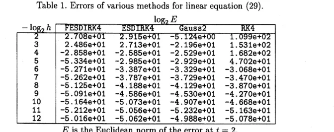
shown in Table 1.

Table 1.

Errors

of various

methods

for linearequation (29).

$\ovalbox{\tt\small REJECT}^{\mathrm{R}\mathrm{K}\mathrm{R}\mathrm{K}}$

$t$

It

can

been

seen

that, although FESDIRK4 is less stable than the tw0-stage Gauss

Runge-Kuttamethodfor larger step-sizes, this method isfitted to the solution completelyfor moderately

small step-sizes; the values of order $-5.0\mathrm{e}+01$

or

less in the second column of Table 1 are due

to the accumulations of round-0ff errors, since the machine epsilon of the arithmetic is $2^{-53}$. On

the other hand, although the other methods are not fitted to this problem completely, the

errors

decrease steadily at the rate of $\mathrm{O}(h^{4})$,

as

expected.

References

[$1_{\rfloor}^{\rceil}$ J. Butcher, The

Numerical

Analysis

of

Ordinary

_Differential

Equations, Wiley,

1987.

[2]

J.R.

Cash,

A

note

on

the exponential fitting

of

blended, extended linear multistep methods,

BIT 21 (1981),

450-454.

[3] J.P. Coleman and S.C. Duxbury, Mixed collocation methods for y” $=f(x,$y), J. Comput.

Appl. Math. 126 (2000), 47-75.

[4] J.M. Franco, Embedded pairs ofexplicit ARKN methods forthe numerical integration of

per-turbed oscillators, Proceedings ofthe 2002 Conference

on

Computational and Mathematical

Methods

on

Science and Engineering CMMSE-2002, (Sep. 2002, at Alicante Spain), Vol1.

92-101.

[5] W. Gautschi, Numerical integration ofordinarydifferential equations based

on

trigonometric

[6] E. Hairer,

S.P.

_Norsett

and

G.

Wanner, Solving Ordinary

Differential

Equations I,

Springer-Verlag,

Second

Revised Edition, 1992.

[7] T.E. Hull, W.H. Enright, B.M. Fellen and A.E. Sedgwick, Comparing numerical methods for

ordinary differential equations, SIAM J. Numer. Anal., 9 (1972),603-637.

[8] N.N. Lebedev, Special Functions

&

Their Applications (Translated

&

edited by R.A.

Silver-man), Dover Publications, Inc. 1972.

[9] B. Neta and C.H. Ford, Families of methods for ordinary differential equations based

on

trigonometric polynomials, J. Computational and Applied Mathematics 10(1984),

33-38.

[10] K. Ozawa, A four-stage implicit Runge-Kutta-Nystr\"om method with variable

coefficients

for

solving periodic initial

value

problems, Japan Journal of

Industrial

and Applied Mathematics,

16 (1999),

25-46.

[11] K. Ozawa, Functional fitting Runge-Kutta method with variable coefficients, Japan Journal

of Industrial and Applied Mathematics 18 (2001),105-128.

[12] K. Ozawa, Functional fitting Runge-Kutta-Nystr\"om methodwithvariablecoefficients, Japan

Journal ofIndustrial and Applied Mathematics 19 (2002),55-85.

[13] K. Ozawa, Functionallyfitted linear multistepmethod, Proceedingsof the2002 Conference on

Computational and Mathematical Methods

on

Science and Engineering CMMSE-2002, (Sep.

2002, at Alicante Spain), VoI I. 271-280.

[14] K. Ozawa, A functionally fitted three-stage explicit singly diagonally implicit Runge-Kutta

method, preprint.

[15] B. Paternoster, Runge-I<utta-Nystr\"om methods for ODEs with periodic solutions based

on

trigonometric polynomials, Applied Numerical Mathematics 28 (1998),

401-412.

[16] $\mathrm{F}.\mathrm{L}.\mathrm{S}\mathrm{h}\mathrm{a}\mathrm{m}\mathrm{p}\mathrm{i}\mathrm{n}\mathrm{e}\mathrm{l}994.$’ Numerical Solution

of

Ordinary

Differential

Equations, Chapman

&

Hall,

[17] E. Stiefel and D.G. Bettis, Stabilization of Cowell’s method, Numer. Math. 13 (1969),

154-175.

[18] T.E. Simos, A fourth algebraic order exponentially-fitted Runge-Kutta method for the

nu-merical solution

of

the Schr\"odinger equation, IMA J. Numer. Anal. 21 (2001), 919-931.

[19] J. Vanthournout, H. De Meyer and

G.

Vanden Berghe, Multistep Methods for Ordinary

Differential

Equations Based

on

Algebraic and First Order Trigonometric Polynomials,

Com-putational Ordinary Differential Equations (Ed. J.R. Cash and I. Gladwell), 1992,

61-71.

[20] G. Vanden Berghe, H. De Meyer, M. Van Daele and T. Van Hecke, Exponentially-fitted

Runge-Kutta methods, Journal of Computational and Applied Mathematics, 125 (2001),

107-115.

[21] P.J. Van Der Houwen and B.P. Sommeijer, Diagonally implicit Runge-Kutta-Nystr\"om_method

ods for oscillatory problems, SIAM J. Numer. Anal. 26 (1989),

414-429.

[22] E.T. Whittaker and

G.N.

Watson, A

Course

_of

ModernAnalysis, Cambridge University Press,

1973.

[8] N.N. Lebedev, Special Functions

&Their

Applicatio\uparrow ls (Translated&edited by R.A.

Silver-man), Dover Publications, Inc. 1972.

[9] B. Neta and C.H. Ford, Families of methods for ordinary differential equations based

on

trigonometric polynomials, J. Computational and Applied Mathematics 10(1984),

33-38.

[10] K. Ozawa, Afour-stage implicit Runge-Kutta-Nystr\"om method with variable

coefficients

for

solving periodic initial

value

problems, Japan Journal of

Industrial

and Applied Mathematics,

16 (1999),

25-46.

[11] K. Ozawa, Functional fitting Runge-Kutta method with variable coefficients, Japan Journal

of Industrial and Applied Mathematics 18 (2001),105-128.

[12] K. Ozawa, Functional fitting Runge-Kutta-Nystr\"om methodwithvariablecoefficients, Japan

Journal ofIndustrial and Applied Mathematics 19 (2002),55-85.

[13] K. Ozawa, Functionallyfitted linear multistepmethod, Proceedingsof the2002 Conference on

Computational and Mathematical Methods

on

Science and Engineering CMMSE-2002, (Sep.

2002, at Alicante Spain), VoI I. 271-280.

[14] K. Ozawa, Afunctionally fitted three-stage explicit singly diagonally implicit $\mathrm{R}\mathrm{u}\mathrm{n}\mathrm{g}\mathrm{e}-\mathrm{I}\acute{\backslash }\mathrm{u}\mathrm{t}\mathrm{t}\mathrm{a}$

method, preprint.

[15] B. Paternoster, Runge-I<utta-Nystr\"om methods for ODEs with periodic solutions based

on

trigonometric polynomials, Applied Numerical Mathematics 28 (1998),

401-412.

[16] F.L. Shampine, Numerical Solution

_of

Ordinary

_Differential

$Equatior|s$, Chapman

&Hall,

1994.

[17] E. Stiefel and D.G. Bettis, Stabilization of Cowell’s method, Numer. Math. 13 (1969),

154-175.

[18] T.E. Simos, Afourth algebraic order exponentially-fitted Runge-Kutta method for the

nu-merical solution

of

the Schr\"odinger equation, IMA J. Numer. Anal. 21 (2001), 919-931.

[19] J. Vanthournout, H. De Meyer and

G.

Vanden Berghe, Multistep Methods for Ordinary

Differential

Equations Based

on

Algebraic and First Order Trigonometric Polynomials,

Com-putational Ordinary Differential Equations (Ed. J.R. Cash and I. Gladwell), 1992,

61-71.

[20] G. Vanden Berghe, H. De Meyer, M. Van Daele and T. Van Hecke, Exponentially-fitted

Runge-Kutta methods, Journal of Computational and Applied Mathematics, 125 (2001),

107-115,

[21] P.J. Van Der Houwen and B.P. Sommeijer, Diagonally implicit Runge-Kutta-Nystr\"om

method

ods for oscillatory problems, SIAM J. Numer. Anal. 26 (1989),

414-429.

$[2\underline{?}]\mathrm{E}.\mathrm{T}$

.

Whittaker and

G.N.

Watson, A

Course

of

ModernAnalysis, Cambridge University Press,