Problems on Low-dimensional Topology, 2019 (Intelligence of Low-dimensional Topology)

全文

(1)117. Problems on Low‐dimensional Topology, 2019 Edited by T. Ohtsuki1. This is a list of open problems on low‐dimensional topology with expositions of their history, background, significance, or importance. This list was made by editing manuscripts written by contributors of open problems to the problem session of the conference “Intelligence of Low‐dimensional Topology” held at Research Institute for Mathematical Sciences, Kyoto University in May 22‐24, 2019.. Contents. 1. Crossing numbers of composite knots and spatial graphs. 2. 2. Correspondence between local moves and invariants of virtual knots. 5. 3. Rectilinear spatial complete graphs. 6. 4. Instanton Floer theory for 3‐manifolds and the homology cobor‐ dism group of integral homology 3‐spheres. 8. 5. The AMU Conjecture for self‐homeomorphisms of surfaces and the volume conjecture for 3‐manifolds 10. 6. The mapping class group of a surface and the quantum invariants of integral homology 3‐spheres 11. 7. Positive flow‐spines and contact 3‐manifolds. 13. lResearch Institute for Mathematical Sciences, Kyoto University, Sakyo‐ku, Kyoto, 606‐8502, JAPAN Email: [email protected]‐u.ac.jp The editor is partially supported by JSPS KAKENHI Grant Numbers. 1. JP16H02145. and. JP16K13754..

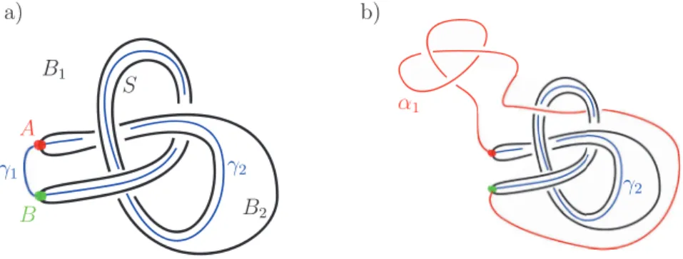
(2) 118 1. Crossing numbers of composite knots and spatial graphs. (Benjamin Bode)2 This section is a collection of problems that relate to the question of the additivity of the crossing number under the connected sum operation, i. e., for two knots K_{1} and K_{2} is c(K_{1}\# K_{2})=c(K_{1})+c(K_{2}) ? This problem is extremely difficult, but the related problems I am going to discuss could give some insights on the crossing number of K_{1}\# K_{2} without us having to tackle the conjecture itself. Malyutin [23] showed that if c(K_{1}\# K_{2})\geq c(K_{1}) for all knots K_{1}, K_{2} or if c(K_{1} \# K_{2})\geq\frac{2}{3}(c(K_{1})+c(K_{2})) for all knots K_{1}, K_{2} , then hyperbolic knots are not generic, meaning that the percentage of hyperbolic knots amongst all of the prime knots of n or fewer crossings approaches 100 as n approaches infinity, a con‐ jecture that was widely believed to be true until then. A positive answer to some of the questions below would disprove this conjecture. Let S\subset S^{3} be diffeomorphic to the standard 2‐sphere S^{2} and denote the two balls that are bounded by S by B_{1} and B_{2} . Let A and B be distinct points on S . For a fixed projection direction we are interested in the number of crossings of a simple path from A to B that lies completely in one of the B_{i}s . We say a path \gamma :. [0,1]arrow B_{i}. with. \gamma(0)=A, \gamma(1)=B. and. \gamma(s)\neq\gamma(t). for all. s\neq t\in[0,1]. minimal in B_{i} if c(\gamma)\leq c(\gamma') for all such paths \gamma' . A minimal path. \gamma_{i}. not be unique (not even up to isotopy). Figure la) shows an example of minimal paths. \gamma_{i}. in B_{i} . We can see that one of them,. a). \gamma_{2} ,. is. in B_{i} might S. and. is isotopic to a path in. S.. b). Figure 1: a) The path \gamma_{1} is minimal in B_{1} with c(\gamma_{1})=0 . The path \gamma_{2} is minimal in B_{2} with c(\gamma_{2})=3 . The path \gamma_{2} is isotopic to a path in S=\partial B_{2}=\partial B_{1} , while \gamma_{1} is not. b) The path \gamma_{2} is minimal in B_{2} with respect to \alpha_{1} with c(\gamma_{2}\cup\alpha_{1})=6 and is isotopic to a path in S.. Question 1.1 (B. Bode). Given S, A, B and a projection direction, is it always true that there is an i\in\{1,2\} and a path \gamma_{i} that is minimal in B_{i} and that is isotopic (with fixed endpoints) to a path in S ‘? 2Department of Mathematics, Osaka University, Toyonaka, Osaka 560‐0043, Japan ben. bode. [email protected]. 2.

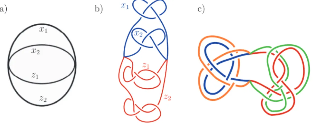
(3) 119 This question becomes more relevant to the additivity of the crossing number if we change the situation slightly. In addition to S, A, B and the fixed projection direction we are now also given two simple paths, \alpha_{i} : [0,1]arrow B_{i} from A to B . We say a simple path \gamma : [0,1]arrow B_{i} from A to B is minimal in B_{i} with respect to \alpha_{j}, j\neq i if c(\gamma\cup\alpha_{j})\leq c(\gamma'\cup\alpha_{j}) for. all such paths \gamma' . An example is depicted in Figure lb).. Question 1.2 (B. Bode). Given S, A, B, \alpha_{i} and a projection direction, is it always true that there is an i\in\{1,2\} and a path \gamma_{i} that is minimal in B_{i} with respect to \alpha_{j}, j\neq i and that is isotopic (with fixed endpoints) to a path in S^{l}? A positive answer to this question would imply that c(K_{1} \# K_{2})\geq\min\{c(K_{1}), c(K_{2})\}. and would therefore show that hyperbolic knots are not generic in the sense of [23]. a). b). c). Figure 2: a) The planar graph \theta^{2}. b ) The spatial graph \theta_{3_{1},4_{1} ^{2}. c ) An element of not \theta_{3_{1},4_{1} ^{2} . Here the constituent knots are 3_{1}\# 4_{1} and 3_{1} (each twice).. \Omega_{3_{1},4_{1} ^{2} , which is. The next question aims at connections between the crossing numbers of composite. knots and spatial graphs as in [4]. Let \theta^{2} be the planar graph with two vertices that are connected by four edges, shown in Figure 2a ). We label the edges by x_{1}, x_{2}, z_{1}. and. z_{2}. in no particular order. Let. \theta_{K_{1},K_{2} ^{2}. be the spatial graph that results from. tying the x ‐edges into the knot K_{1} and the z ‐edges into K_{2} as in Figure. 2b ).. The. unions of any pair of distinct edges of this spatial graph form knots, the constituent knots of the spatial graph, namely either K_{1}\# K_{2} ( x_{i} with z_{j} ), K_{1}\# K_{1} ( x_{i} with x_{j} ) or K_{2}\# K_{2} ( z_{i} and z_{j} ). Let \Omega_{K_{1},K_{2} ^{2} be the set of isotopy classes of embeddings of \theta^{2} such that its constituent knots are as follows: \bullet. \bullet. x_{i}\cup z_{j}=K_{1}\# K_{2}. for all i,. j=1,2,. x_{i}\cup x_{j}=K_{1}\# K_{1} and z_{i}\cup z_{j}=K_{2}\# K_{2} or both are prime. (In particular, they are not unknots.). From this definition it is clear that. \theta_{K_{1},K_{2} ^{2}\in\Omega_{K_{1},K_{2} ^{2}.. Question 1.3 (B. Bode). Is c(\theta_{K_{1},K_{2}})\leq c(\Gamma) for all \Gamma\in\Omega_{K_{1},K_{2}^{\beta)} ^{2}. 3.

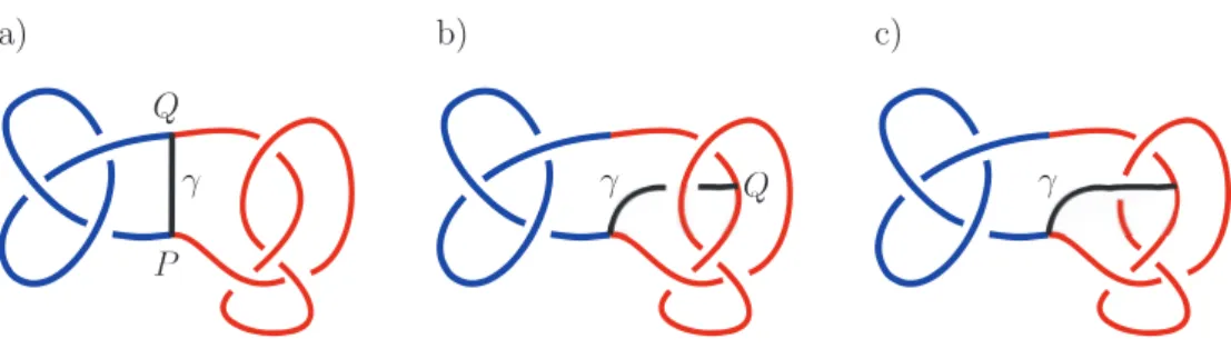
(4) 120 It follows from [4] that a positive answer to this question would imply that. c(K_{1} \# K_{2})\geq\frac{1}{4}(c(K_{1}\# K_{1})+c(K_{2}\# K_{2}) . Note that we do not know. 2b). is minimal.. a). (1). c(\theta_{K_{1},K_{2} ^{2}) ,. since we do not know if the diagram in Figure. b). c). Figure 3: a) For this choice of P and Q the black arc \gamma minimizes c(D') because it does not add any crossings to D . The constituent knots of this theta curve are 3_{1}\# 4_{1},3_{1} and 4_{1} . b) For a different choice of P and Q the black curve has to intersect D somewhere. The shown arc does so the minimal number of times possible. The constituent knots of this theta curve are 3_{1}\# 4_{1},3_{1} and 4_{1}. c) Changing the signs of crossings between the black arc and the diagram D does not change the fact that \gamma minimzes c(D') for this choice of endpoints P and Q . It can change the constituent knots however. Here they are 3_{1}\# 4_{1},3_{1} and the unknot.. Let D be a knot diagram of a composite knot K_{1}\# K_{2} . Pick an arbitrary point on D . For any additional point Q on D any simple path \gamma from P to Q that does not intersect K_{1}\# K_{2} turns the knot diagram into a diagram D'=D\cup\gamma of a spatial graph (a theta‐curve \theta ), one of whose constituent knots is K_{1}\# K_{2}. Let \gamma' be a path that minimizes c(D') among all simple paths from P to Q that do not intersect K_{1}\# K_{2} . Again this minimizer is usually not unique. An example for two different choices of P and Q , where D is the minimal diagram of 3_{1}\# 4_{1} is given in Figure 3. P. Question 1.4 (B. Bode). Given any diagram. D of K_{1}\# K_{2} , does there exist a choice of P and Q such that there is a simple path \gamma' from P to Q that does not intersect K_{1}\# K_{2} , that minimizes c(D') and such that the constituent knots of \theta are K_{1}\# K_{2},. K_{1} and K_{2} ?. A positive answer to this question would imply that c(K_{1} \# K_{2})>\frac{2}{3}(c(K_{1})+c(K_{2})) and therefore also show that the conjecture on the genericity of hyperbolic knots is. false [23].. 4.

(5) 121 121. 2. Correspondence between local moves and invariants of virtual knots. (Shin Satoh3) The set of welded knots is a quotient of the set of virtual knots, by the move. “overcrossings commute” It is known (see [37]) that the set of classical knots is a. proper subset of the set of welded knots, and hence a proper subset of virtual knots. Some invariants of classical knots correspond to some local moves in the sense that two classical knots have the same invariant if and only if they are related by a. finite sequence of the local moves; see e.g. [34, Section 2.8]. For example, the Arf invariant of a classical knot corresponds to pass moves [19, 20]. It is important to study such correspondence because it reveals a relationship between algebraic and geometric structures in classical knot theory. From this point of view, there are many problems according to which family of knots, which invariant of knots, and which local moves for knots we choose. For example, the delta move, pass move, and sharp move are known to be unknotting. operations for welded knots [40], but not unknotting operations for virtual knots [41].. \tilde{I^\backsla h}\gam a_{)\nearow}rightarow/\backsla h\frac{1} {\prime_{\backsla h} delta move. rightar owar ow^{\upar ow\upar ow 1 }. arrow. rightar owar ow^{|11\upar ow}. arrow. | \downarrow 1. sharp move. pass move. \mu ‐component. virtual link (\mu\geq 1) corresponding. Problem 2.2. Find invariants of a to the pass move.. \mu ‐component. virtual link (\mu\geq 1) corresponding. Problem 2.3. Find invariants of a to the sharp move.. \mu ‐component. virtual link (\mu\geq 1) corresponding. Problem 2.4. Find invariants of a. \mu ‐component. welded link (\mu\geq 2) corresponding. Problem 2.5. Find invariants of a to the pass move.. \mu ‐component. welded link (\mu\geq 2) corresponding. Problem 2.6. Find invariants of a to the sharp move.. \mu ‐component. welded link (\mu\geq 2) corresponding. Problem 2.1. Find invariants of a to the delta move.. to the delta move.. In virtual knot theory, there are several invariants such as the n ‐writhe (n\neq 0) , the writhe polynomial, the odd writhe, the r ‐covering (r\geq 0, r\neq 1)[29] , and the Jones polynomial. 3Department of Mathematics, Kobe University, Rokkodai‐cho 1‐1, Nada‐ku, Kobe 657‐8501, Japan Email address: [email protected]‐u.ac.jp. 5.

(6) 122 Problem 2.7. Find local moves for a virtual knot corresponding to the. (n\neq 0). n. ‐writhe. .. Problem 2.8. Find local moves for a virtual knot corresponding to the. (r\geq 0, r\neq 1). r. ‐covering. .. Problem 2.9. Find local moves for a ing to the Jones polynomial.. \mu ‐component. virtual link (\mu\geq 1) correspond‐. It is known that the odd writhe of a virtual knot corresponds to a local move. called the \Xi ‐move [41] and the writhe polynomial corresponds to a local move called the shell move (given in our talk of this conference). We find several invariants corresponding to the shell move in the case of a 2‐component virtual link [30]. In the figure, the real crossings with the same label have the same crossing information.. rightarrow --- ‐move. Problem 2.10. Find invariants for a ing to the :‐move.. \mu ‐component. virtual link (\mu\geq 2) correspond‐. Problem 2.11. Find invariants for a ing to the shell move.. \mu ‐component. virtual link (\mu\geq 3) correspond‐. There is known no skein relation for the odd writhe and writhe polynomial of a virtual knot.. Problem 2.12. Find a skein relation for the odd writhe of a virtual knot.. Problem 2.13. Find a skein relation for the writhe polynomial of a virtual knot.. 3. Rectilinear spatial complete graphs. (Ryo Nikkuni)4 An embedding f of a finite graph G into \mathbb{R}^{3} is called a spatial embedding of G, and the image f(G) is called a spatial graph of G . We call a subgraph \gamma of G homeomorphic to the circle a cycle of G , and also call a k ‐cycle if it contains exactly k edges. We denote the set of all k ‐cycles of G by \Gamma_{k}(G) , and the set of all pairs of two disjoint cycles of G consisting of a k ‐cycle and an l ‐cycle by \Gamma_{k,l}(G) . For a cycle \gamma (resp. a pair of disjoint cycles \lambda ) and a spatial embedding f of G, f(\gamma) (resp.. f(\lambda)) is none other than a knot (resp. a 2‐component link) in f(G) . For a cycle G containing all vertices of G , we call f(\gamma) a Hamiltonian knot in f(G) .. \gamma. of. 67-8585,Japan4 Suginami-ku, fMa.. jppukuji, Department otwcuTokyo tahematil cs,School o Email:nick@lab.. c.. fArts. and Sciences, Tokyo Woman’s Christian University, 2‐6‐1 Zem‐ 6.

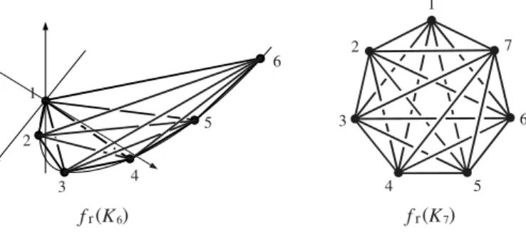
(7) 123 Let K_{n} be the complete graph on n vertices, that is the graph consisting of n vertices such that each pair of its distinct vertices is connected by exactly one edge. A spatial embedding f_{r} of K_{n} is said to be rectilinear if for any edge e of K_{n}, f_{r}(e) is a straight line segment in \mathb {R}^{3} . Such an embedding can be constructed by taking n vertices of K_{n} on the moment curve (t, t^{2}, t^{3}) in \mathbb{R}^{3} and connecting every pair of two. distinct vertices by a straight line segment, see Figure 4 for n=6,7 (we say such a rectilinear spatial graph of K_{n} is standard). As a consequence of generalizations of the Conway‐Gordon theorems [8], Morishita‐Nikkuni showed the following formula. Theorem ([26]). Let of K_{n} , we have. n\geq 6. be an integer. For any rectilinear spatial embedding f_{r}. \sum_{\gamma\in\Gamma_{n}(K_{n}) a_{2}(f_{r}(\gamma) =\frac{(n-5)!}{2} ( \sum_{\lambda\in\Gam a_{3, }(K_{n}) lk (f_{r}(\lambda))^{2}- (\begin{ar y}{l n -1 5 \end{ar y}) ), where lk denotes the linking number, and Conway polynomial.. a_{2}. denotes the second coefficient of the. fr(K_{6}) f_{r}(K_{7}) Figure 4:. Standard rectilinear spatial graphs of K_{n}(n=6,7). Note that every polygonal 2‐component link with exactly six sticks is either a trivial link or a Hopf link. Thus \sum_{\lambda\in\Gamma_{3,3}(K_{n})} lk (f_{r}(\lambda))^{2} coincides with the number of “triangle‐triangle” Hopf links in f_{r}(K_{n}) . The original Conway‐Gordon theorem for K_{6} implies that \sum_{\lambda\in\Gamma_{3,3}(K_{n})} lk (f_{r}(\lambda))^{2} is greater than or equal to the number of. subgraphs of K_{n} isomorphic to K_{6} , that is equal to (\begin{ar y}{l n 6 \end{ar y}) . On the other hand, it is known that every rectilinear spatial graph of K_{6} contains at most three Hopf links. [17, 16, 31]. This implies that \sum_{\lambda\in\Gamma_{33}(K_{n})} lk (f_{r}(\lambda))^{2} is less than or equal to 3 (\begin{ar y}{l n 6 \end{ar y}) . Thus by the theorem, we have the folíowing evaluations of the “algebraic” number of Hamiltonian knots in every rectilinear spatial graph of K_{n}.. Corollary ([26]). Let n\geq 6 be an integer. For any rectilinear spatial embedding f_{r} of K_{n} , we have. \frac{(n-5)(n-6)(n-1)!}{2\cdot 6!}\leq\sum_{\gamma\in\Gamma_{n}(K_{n})}a_{2} (f_{r}(\gamma) \leq\frac{3(n-2)(n-5)(n-1)!}{2\cdot 6!}. 7.

(8) 124. The lower bound in the corollary is sharp for arbitrary n\geq 6[26] . Actually the standard rectilinear spatial graph of K_{n} realizes the sharp lower bound. In the case of n=6 , the upper bound 1 is also sharp. On the other hand, the upper bound in. the case of. n=7. is 15, but according to a computer search in [18], there seems to. be no rectilinear spatial embedding f_{r} of K_{7} such that \sum_{\gamma\in\Gamma_{7}(K_{7})}a_{2}(f_{r}(\gamma))=13,15. This strongly suggests that the upper bound in the corollary is not sharp.. Problem 3.1 (R. Nikkuni). Determine the sharp upper bound of for all rectilinear spatial embeddings f_{r} of K_{n} for each n\geq 7.. \sum_{\gamma\in\Gamma_{n}(K_{n})}a_{2}(f_{r}(\gamma)). By the above mentioned theorem, Problem 3.1 is equivalent to the following problem.. Problem 3.2 (R. Nikkuni). Determine the maximum number of triangle‐triangle Hopf links in f_{r}(K_{n}) for all rectilinear spatial embeddings f_{r} of K_{n} for each n\geq 7.. 4. Instanton Floer theory for 3‐manifolds and the homology cobordism group of integral homology 3‐spheres. (Yuta Nozaki, Kouki Sato, Masaki Taniguchi) Instanton Floer theory. The instanton Floer homology group I_{*}(Y) is an invariant of an oriented integral. homology 3‐sphere. Y. introduced by Floer [13]. The group I_{*}(Y) is an analog of. infinite dimensional Morse homology with respect to the Chern‐Simons functional. We denote by \Omega^{1}(Y)\otimes \mathfrak{s}u(2) the set of \mathfrak{s}u(2) ‐valued 1‐forms. The Chern‐Simons functional cs(a) is given by. cs(a):= \frac{1}{8\pi^{2} \int_{Y} (a \wedge da+\frac{2}{3}a\wedge a\wedge a) Tr. .. If we fix a Riemann metric g on Y , one can consider the formal gradient of cs with respect to an L^{2} ‐metric. There is a large symmetry on \Omega^{1}(Y)\otimes su(2) which is called null‐homotopic gauge symmetry defined by. \mathcal{G}_{Y} :=\{g\in Map(Y, SU(2))|\deg(g)=0\}, where the degree is the mapping degree. The action is given by One can see the map cs descends to the map cs. a\cdot g. :=g^{-1}dg+g^{-1}ag.. :\mathcal{B}_{Y}:=(\Omega^{1}(Y)\otimes \mathfrak{s}u(2) /\mathcal{G}_{y}arrow \mathbb{R}.. The set of solution to F(a)=0 in \mathcal{B}_{y} is denoted by R_{Y} . Some parts of R_{Y} correspond to critical values of cs. In a good situation, the chains are generated by some part of R_{Y} . The differential is defined by counting the solution to the gradient flow of cs. The gradient flows correspond to solutions to ASD‐equation on Y\cross \mathbb{R}. Although the group I_{*}(Y) is the first example of Floer homology groups for 3‐ manifolds, even the following fundamental problem is still open. 8.

(9) 125 Problem 4.1. Construct a well‐defined equivariant instanton Floer homology for SU(2) ‐bundles on all 3‐manifolds. The main problems are to deal with the reducible solutions and the dependence. of perturbations. For example, the dependence of perturbations made in [2] is still open. We also mention a problem related to Floer homotopy types introduced in [7].. It is known that several Floer theoretical invariants of 3 or 4‐manifolds are obtained. as the singular homology of some topological objects, and the stable homotopy types of the topological objects themselves are invariants of 3 or 4‐manifolds. Thus, the. homotopy type is called the Floer homotopy type ([24, 22]). For the group I_{*}(Y) , its Floer homotopy type has been unknown.. Problem 4.2. Construct a Floer homotopy type of I_{*}(Y) . The main problems to define an instanton Floer homotopy type are related to the bubble phenomena and the existence of structures of manifolds with corners on the compactification of moduli spaces of trajectories and the framings. If the problem is solved, we can apply a generalized cohomology theory and obtain a family of invariants.. Homology cobordism group. Two oriented integral homology 3‐spheres Y_{1}, Y_{2} are homology cobordant if there exists a cobordism W from Y_{1} to Y_{2} with. H_{*}(W;\mathbb{Z})\cong H_{*}(S^{3}\cross I;\mathbb{Z}) .. This is an. equivalence relation on the set of oriented integral homology 3‐spheres, and the quotient set \Theta^{3} equipped with the connected sum operation is an abelian group. called the homology cobordism group. It is known [12, 14] that \Theta^{3} contains a. \mathbb{Z}^{\infty}. The group \Theta^{3} has. subgroup, which is generated by Seifert homology 3‐spheres. further been studied since various Floer theory for 3‐manifolds were established, while we still have several elementary open problems. For instance, the following question is open.. Question 4.3. Denote by \Theta_{S}^{3} the subgroup of \Theta^{3} generated by Seifert homology 3‐spheres. Then, is the quotient group \Theta^{3}/\Theta_{S}^{3} non‐trivial!? Here we mention that the above question is related to our invariant r_{+}:\Theta^{3}arrow. \mathbb{R}_{\geq 0}\cup\{\infty\} ; for details of. r+ ,. see [32]. In fact, the value r_{+}(Y) is contained in cs(R_{Y}) ,. and if Y is a linear combination of Seifert homology 3‐spheres, then cs(R_{Y})\subset \mathbb{Q}. These imply that if a homology 3‐sphere Y has irrational r+ , then its homology cobordism class [Y] is not contained in \Theta_{S}^{3} . On the other hand, by Mathematica, the authors estimated the value r_{+}(S_{1/2}^{3}(5_{2}^{*})) with an error of at most 10^{-46} , where. S_{1/2}^{3}(5_{2}^{*}) denotes the 3‐manifold obtained by 1/2‐surgery on the mirror of the knot noting that S_{1/2}^{3}(5_{2}^{*}) is a hyperbolic 3‐manifold (see [5]). The result seems to imply that r_{+}(S_{1/2}^{3}(5_{2}^{*})) is irrational. If the value r_{+}(S_{1/2}^{3}(5_{2}^{*})) is truly irrational, then we can conclude that [S_{1/2}^{3}(5_{2}^{*})]\not\in\Theta_{S}^{3}. Question 4.4 (Y. Nozaki, K. Sato, M. Taniguchi). Is the value r_{+}(S_{1/2}^{3}(5_{2}^{*})) irra‐ 5_{2} ,. tional;?. 9.

(10) 126 The method of our computation is based on Kirk and Klassen’s formula of cs given by the integration along a path in the space of irreducible SL(2, \mathbb{C}) ‐representations. To obtain the approximate value of r+ , we use a description of the space of SL(2, \mathbb{C}) ‐. representations of \pi_{1}(S^{3}\backslash 5_{2}) , as in [36], in terms of a Riley polynomial \phi(t, u)\in \mathbb{Z}[t^{\pm 1}, u] with \deg_{u}\phi=3 . Then we can explicitly solve the equation \phi(u, t)=0. with respect to u and use the solutions to compute r+\cdot However, Riley polynomials \phi(t, u) of 2‐bridge knots K might be of degree larger than 4. In this case, one cannot solve \phi(t, u)=0 in general.. Problem 4.5 (Y. Nozaki, K. Sato, M. Taniguchi). In the case \deg_{u}\phi>4 , give a method to compute an approximate value of. r_{+}(S_{1/n}^{3}(K)) .. Note that, in principle, we can compute approximate values by dividing a path into shorter paths.. 5. The AMU Conjecture for self‐homeomorphisms of sur‐ faces and the volume conjecture for 3‐manifolds. (Tian Yang) According to Nielsen‐Thurston’s classification of the elements of the mapping class group of surfaces, every irreducible orientation preserving self‐homeomorphism. of a surface of finite type is either periodic (of finite order) or pseudo‐Anosov (pre‐ serving two transverse measure laminations). Here a self‐homeomorphism being irreducible means that it does not restrict of a proper subsurface. In [1], Andersen‐ Masbaum‐Ueno made the following. Conjecture 5.1 (J. E. Andersen, G. Masbaum, K. Ueno [1]). Let. \Sigma. be. a. orientable. surface of finite type, let \phi be a pseudo‐Anosov self‐homeomorphism of \Sigma , and let \{\rho_{r}\}_{r} be the sequence of the Turaev‐ Viro representations of the mapping class group of \Sigma . Then for r sufficiently large, \rho_{r}([\phi]) is a linear transformation of infinite order. Combined with the fact that the image of a finite order element under any group representation is of finite order, the AMU Conjecture essentially claims that the sequence of Turaev‐Viro representations of the mapping class groups respects the Nielsen‐Thurston classification. The similar conjecture can be made for the Reshetikhin‐ Turaev representations, which are a sequence of projective representations of map‐ ping class group of surfaces. The AMU conjecture is known to be true for punctured. spheres [1, 11] and the once‐punctured torus [38]. Recently, Marché‐Santharoubane [25] related the Turaev‐Viro representations to representations of the fundamental group of surfaces, and provide an efficient algorithm of determining whether an element of the fundamental group can be represented by a simple closed curve on the surface, assuming that the AMU Conjecture is true.. Observed by Santharoubane [39] (see also Detcherry‐Kalfagianni [10]), the AMU. Conjecture is a consequence of the following a weaker version of the Volume Con‐. jecture of Chen‐Yang [6]. 10.

(11) 127 Conjecture 5.2 (a weaker version of the volume conjecture of Q. Chen and T. Yang [6]). Let M be a hyperbolic 3‐manifold with finite volume, and let TV_{r}(M;q) be its r‐th Turaev‐ Viro invariant at the root of unity q . Then for the odd integers,. r. running over all. 1 \dot{ \imath} m\dot{ \imath} nf\frac{1}{r}\ln TV_{r}(M;e^{\frac{2\pi }{r} )r \mapsto\infty>0.. The relationship between the two conjectures mentioned above is given by the under‐ lying TQFTs. Roughly speaking, the mapping cylinder MC_{\phi} of \phi can be considered as a cobordism from \Sigma to itself. Hence for each r , the Turaev‐Viro TQFT assigns MC_{\phi} a linear map, which is exactly \rho_{r}([\phi]) by the construction of the Turaev‐Viro representation. By the TQFT axioms, the trace of \rho_{r}([\phi]) equals to the Turaev‐ Viro invariant TV_{r}(M_{\phi}) of the mapping torus M_{\phi} of \phi . Since \phi is pseudo‐Anosov, Thurston’s result shows that M_{\phi} is hyperbolic. Then Conjecture 5.2 implies that TV_{r}(M) grows at least exponentially at particular roots of unity. On the other hand, if \rho_{r}([\phi]) was of finite order, the each of its eigenvalues should be a root of unity. As a consequence, the trace of \rho_{r}([\phi]) is at most the dimension of the TQFT vector space of \Sigma , which by the Verlinde formula is only a polynomial in r . That is a contradiction.. In a recent work [9], Detcherry‐Kalfagianni showed that the behavior of the Turaev‐Viro invariant is “similar to” that of the hyperbolic volume, in the sense that it does not increase under Dehn‐fillings. Therefore, if one could prove Conjec‐ ture 5.2 for a 3‐manifold M , then Conjecture 5.2 is automatically true for all the. 3‐manifolds obtained from M by removing a link inside it. Recently, Ohtsuki [35] and Belletti‐Detcherry‐Kalfagianni‐Yang [3] proved the Volume Conjecture of Chen‐ Yang for infinite families of 3‐manifolds, including the closed hyperbolic ones ob‐ tained by doing integral Dehn‐fillings along the figure‐8 knot and the fundamental shadow link complements. Therefore, Conjecture 5.2 hold for all the 3‐manifolds obtained from the examples mentioned above by remove a link inside them, and the AMU Conjecture holds for the fibered ones obtained from those examples by doing the same operation. From the discussions above, one sees that a solution to the follow problem will give a final solution to the AMU Conjecture, at least for all the punctured surfaces.. Problem 5.3 (T. Yang). Find a family of 3‐manifolds for which Conjecture 5.2 holds, and by removing links from which one gets all the pseudo‐Anosov mapping torus of all punctured surfaces.. 6. The mapping class group of a surface and the quantum invariants of integral homology 3‐spheres. (Shunsuke Tsuji) Let \Sigma_{g,1} be a surface of genus 1 with a connected non‐empty boundary. We con‐ sider the lower central series \{F^{n}\pi_{1}(\Sigma_{g,1}, *)\}_{n\geq 1} of \pi_{1}(\Sigma_{g,1}, *) where *\in\partial\Sigma_{g,1} , de‐ fined by. F^{1}\pi_{1}(\Sigma_{g,1}, *)^{def}=\pi_{1}(\Sigma_{g,1}, *) and F^{n+1}\pi_{1}(\Sigma_{g,1}, *)=def[\pi_{1}(\Sigma_{g,1}, *), F^{n}\pi_{1} (\Sigma_{g,1}, *)]. 11.

(12) 128 We denote by \mathcal{M}(\Sigma_{g,1}) the mapping class group of \Sigma_{g,1} and by \mathcal{I}(\Sigma_{g,1}) the Torelli group, which is the kernel of the action of \mathcal{M}(\Sigma_{g,1}) on the homology group of. \Sigma_{g,1} .. We can define two filtrations. \{\mathcal{I}^{(n)}(\Sigma_{g,1})\}_{n\geq 1}. \{\mathcal{I}^{(n)}(\Sigma_{g,1})\}_{n\geq 1}. and. is the lower central series, defined by. \mathcal{I}^{(n+1)}(\Sigma_{g,1})=def[\mathcal{I}(\Sigma_{g,1}),\mathcal{I} ^{(n)}(\Sigma_{g,1})] .. tration, satisfying. \mathcal{M}^{(n)}(\Sigma_{g,1}). F^{1}\pi_{1}(\Sigma, *)/F^{n+1}\pi_{1}(\Sigma, *). The second. \{\mathcal{M}^{(n)}(\Sigma_{g,1})\}_{n\geq 1} .. The first. \mathcal{I}^{(1)}(\Sigma_{g,1})def=\mathcal{I}(\Sigma_{g,1}). \{\mathcal{M}^{(n)}(\Sigma_{g,1})\}_{n\geq 1}. and. is the Johnson fil‐. is the kernel of the action of \mathcal{M}(\Sigma_{g,1}) on. .. We denote by. z^{s1_{2}}(M)=1+z_{1}^{s1_{2}}(M)(q-1)+z_{2}^{s1_{2}}(M)(q-1)^{2}+\cdots the invariant of an integral homology 3‐sphere. M. defined by T. Ohtsuki [33]. We fix. S^{3}=H_{g}^{+} \bigcup_{\iota}H_{g}^{-} , where H_{g}^{+} and H_{g}^{-} are handle bodies of genus is a diffeomorphism from \partial H_{g}^{+} to \partial H_{g}^{-} . We denote M( \psi)def=H_{g}^{+}\bigcup_{\psi\circ\iota}H_{g}^{-} g and for \psi\in \mathcal{M}(\Sigma_{g,1}) , where we consider \Sigma_{g,1} as a submanifold of \partial H_{g}^{+}. Then we obtain z_{i}^{s1_{2}}(M(\psi))=0 if \psi\in \mathcal{I}^{(2i+1)}(\Sigma_{g,1}) for any i . In the case of the Johnson filtration \{\mathcal{M}^{(n)}(\Sigma_{g,1})\}_{n\geq 1} , there exists \psi\in \mathcal{M}^{(3)}(\Sigma_{g,1}) satisfying z_{1}^{s1_{2}}(M(\psi))\neq 0 . S. Morita [27] constructs the core of the Casson invariant d : \mathcal{M}^{(2)}(\Sigma_{g,1})arrow \mathbb{Z} where z_{1}^{s1_{2}}(M(\psi))=0 if \psi\in \mathcal{I}^{(3)}(\Sigma_{g,1})\cap kerd . In other words, we can define z_{1}^{s1_{2} using the Johnson homomorphisms and the core of the Casson a Heegaard splitting of \iota. invariant.. Conjecture 6.1 (S. Morita). For any i\in \mathbb{Z}_{\geq 1}, z_{i}^{s{\imath}_{2}}(M(\psi))=0if\psi\in \mathcal{M}^{(2i+1)}(\Sigma_{g,1}) \cap kerd.. By definition, if. i=1 ,. the conjecture is true.. Morita-Sakasai- Suzuki. [ 28] prove that. the conjecture is true if i=2,3. We can also define. z^{s1_{N}}(M)=1+z_{1}^{s1_{N}}(M)(q-1)+z_{2}^{s1_{N}}(M)(q-1)^{2}+\cdots using the s1_{N} ‐quantum group in [21]. Conjecture 6.2 (S. Morita, S. Tsuji). Fix an integer i\in \mathbb{Z}_{\geq 1}, z_{i}^{s1_{N}}(M(\psi))=0 if \psi\in \mathcal{M}^{(2i+1)}(\Sigma_{g,1})\cap kerd. By definition, if. i=1 ,. N. larger than 2. For any. the conjecture is true. Morita‐Sakasai‐Suzuki [28] also prove. that the conjecture is true if i=2,3. We introduce an approach of the conjectures using skein algebras. Let \{\mathcal{M}_{Kauffman}^{(n)}(\Sigma_{g,1})\}_{n\geq 1} be a filtration of the Torelli group defined using the Kauff‐ man bracket skein algebra. For any i\in \mathbb{Z}_{\geq 1} , we have z_{i}^{s1_{2}}(M(\psi))=0 if \psi\in \mathcal{M}_{Kauffman}^{(2i+1)}(\Sigma_{g,1}) . If \mathcal{M}^{(i)}(\Sigma_{g,1})\cap kerd\subset \mathcal{M}_{Kauffman}^{(i)} (\Sigma_{g,1}) for any i , the first con‐. jecture is true. Let \{\mathcal{M}_{HOMFLy-PT}^{()}(\Sigma_{g,1})\}_{n\geq 1} be a filtration of the Torelli group defined using the HOMFLY‐PT skein algebra. For any N and any i\in \mathbb{Z}_{\geq 1} , we have. \psi\in \mathcal{M}_{HOMFLY-PT}^{(2x+1)}(\Sigma_{g,1}) . We remark that \mathcal{M}^{(i)}(\Sigma_{g,1})\cap kerd\supset \mathcal{M}_{HOMFLY-PT}^{(i)}(\Sigma_{g,1}) . If \mathcal{M}^{(i)}(\Sigma_{g,1})\cap kerd=\mathcal{M}_{HOMFLY-PT}^{(i)} (\Sigma_{g,1}) for any i , the second z_{i}^{s1_{N}}(M(\psi))=0. if. conjecture is true for any. N.. 12.

(13) 129 7. Positive flow‐spines and contact 3‐manifolds. (Ippei Ishii, Masaharu Ishikawa, Yuya Koda, Hironobu Naoe) In this section,. M. always denotes a closed, oriented, smooth 3‐manifold.. (positive) contact structure on M is a transversely orientable 2‐plane field on M , given as the kernel of a 1‐form (called a contact form) \alpha on M , where a satisfies \alpha\wedge d\alpha>0 . The pair (M, \xi) is called a contact 3‐manifold. Two contact A. structures \xi_{0} and \xi_{1} are said to be isotopic if there exists a 1‐parameter family of contact structures connecting them. For a contact form \alpha , the Reeb vector field R_{\alpha} is defined by d\alpha(R_{\alpha}, \cdot)=0 and \alpha(R_{\alpha})=1 . We also call R_{\alpha} a Reeb vector field of the contact structure \xi=ker\alpha . The flow generated by R_{\alpha} is called the Reeb flow of \alpha (or a Reeb flow of \xi ). A contact structure \xi is said to be overtwisted if there exists a disk D embedded in M such that \partial D is everywhere tangent to \xi and the framing of D along \partial D coincides with that of \xi . Otherwise \xi is said to be tight. A 2‐dimensional polyhedron P in M is called a flow‐spine if. (1). P. is a spine, that is, M\backslash P is an open 3‐ball; and. (2) there exists a non‐singular flow \Phi=\{\varphi_{t}\}_{t\in \mathbb{R} on M such that for each point of P , there exists a positive chart (U;x, y, z) of M around the point such that (U, U\cap P) is diffeomorphic (by an orientation‐preserving diffeomorphism) to one of the four models shown in Figure 5, where the flow by the vector field \partial/\partial z. Further, a flow‐spine. P. is said to be positive if. P. \Phi. on. U. is generated. has at least one point of the model. of Figure 5 (iii) and has no point of the model of Figure 5 (iv). In the above setting,. we say that the flow \Phi is carried by P . A contact structure \xi on supported by a flow‐spine P if a Reeb flow of \xi is carried by P.. M. is said to be. z_{L_{ar ow}^{y}. x. (i). (ii). (iii). (iv). Figure 5: The ıocal models of a flow‐spine.. Theorem (I. Ishii, M. Ishikawa, Y.Koda, H. Naoe). The map. {positive flow‐spines of M}/isotopy. arrow. {contact structures on M}/isotopy. that takes a positive flow‐spine P (up to isotopy) to a contact structure \xi (up to isotopy) whose Reeb flow is carried by P is a well‐defined surjective map.. 13.

(14) 130 Problem 7.1 (I. Ishii, M. Ishikawa, Y.Koda, H. Naoe). Find moves for positive flow‐spines so that the map. {positive flow‐spines of. M}. /movesarrow {contact structures on M}/isotopy. induced from the surjection in the theorem is a bijection.. Apparently, an answer to the above problem completes to give a counterpart of the. famous Giroux correspondence [15]. In the Giroux correspondence, it is known that a contact 3‐manifold (M, \xi) is Stein fillable if and only if (M, \xi) admits a supporting open book decomposition whose monodromy is a product of right‐handed Dehn twists. In particular, \xi is tight in this case.. Problem 7.2 (I. Ishii, M. Ishikawa, Y.Koda, H. Naoe). Give a criterion for the tightness or Stein fillability of contact structures in terms of supporting positive flow‐spines. It is known that for any non‐singular flow \Phi on M , there exists a flow‐spine carrying \Phi . Further, by the above mentioned theorem, a certain Reeb flow of any contact manifold (M, \xi) is carried by a positive flow‐spine.. Question 7.3 (I. Ishii, M. Ishikawa, Y.Koda, H. Naoe). Is any Reeb flow of any contact manifold (M, \xi) carried by a positive flow‐spine /? A point of a flow‐spine. P. whose neighborhood is shaped on the model (iii) in. Figure 5 is called a vertex of P . The complexity c(M, \xi) of a contact 3‐manifold (M, \xi) is defined to be the minimum number of vertices of any positive flow‐spine supporting \xi . Note that c is finite‐to‐one. The classification of contact 3‐manifolds of complexity up to 3 is now in progress.. Problem 7.4 (I. Ishii, M. Ishikawa, Y.Koda, H. Naoe). ClassOfy the contact 3‐ manifolds of complexity 4. In our classification, it seems that any positive flow‐spine with at most 3 vertices sup‐ ports a tight contact structure. On the other hand, there exists a positive flow‐spine of S^{3} with 5 vertices supporting an overtwisted contact structure. It is interesting to determine whether there is a positive flow‐spine with 4 vertices supporting an overtwisted contact structure or not.. References [1] Andersen, J. E., G. Masbaum, G., Ueno, K., Topological quantum field theory and the Nielsen‐ Thurston classification of M(0, 4) , Math Proc. Cambridge Philos. Soc. 141 (2006) 477‐488. [2] Austin, D. M., Braam, P. J., Equivariant Floer theory and gluing Donaldson polynomials Topology 35 (1996) 167‐200. [3] Belletti, G., Detcherry, R., Kalfagianni, E., Yang, T., Growth of quantum 6\dot{j} ‐symbols and applications to the Volume Conjecture, GT. arXiv:lS07.03327. [4] Bode, B., Crossing numbers of composite knots and spatial graphs, Topology and its Applica‐ tions 243 (2018) 33‐51. 14.

(15) 131 131 [5] Brittenham, M., Wu, Y.‐Q., The classification of exceptional Dehn surgeries on 2‐bridge knots, Comm. Anal. Geom. 9 (2001) 97‐113. [6] Chen, Q., Yang, T., Volume conjectures for the Reshetikhin‐Turaev and the Turaev‐Viro in‐ variants, Quantum Topol. 9 (2018) 419‐460. [7] Cohen, R. L., Jones, J. D. S., Segal, G. B., Floer’s infinite‐dimensional Morse theory and homotopy theory, The Floer memorial volume, 297‐325, Progr. Math., 133, Birkhauser, Basel, 1995.. [8] Conway, J. H., Gordon, C. McA., Knots and links in spatial graphs, J. Graph Theory 7 (1983) 445‐453.. [9] Detcherry, R., Kalfagianni, E., Gromov norm and Turaev‐Viro invariants of 3‐manifolds, Ann. Sci. de l’Ecole Normale Sup., to appear.. [10] —, Quantum representations and monodromies of fibered links, GT. arXiv:1711.03251.. [11] Egsgaard, J. K., Jorgensen, S. F., The homological content of the jones representations at q −1, Journal of Knot Theory and its ramifications 25 (2016), no. 11, 25pp. =. [12] Fintushel, R., Stern, R. J., Instanton homology of Seifert fibred homology three spheres, Proc. London Math. Soc. (3) 61 (1990) 109‐137. [13] Floer, A., An instanton‐invariant for 3‐manifolds, Comm. Math. Phys. 118 (1988) 215‐240.. [14] Furuta, M., Homology cobordism group of homology 3‐spheres Invent. Math. 100 (1990) 339‐ 355.. [15] Giroux, E., Géométrie de contact: de la dimension trois vers les dimensions supérieures, Proceedings of the International Congress of Mathematicians, Vol. II (Beijing, 2002), 405‐ 414, Higher Ed. Press, Beijing, 2002.. [16] Huh, Y., Jeon, C., Knots and links in linear embeddings of K_{6} , J. Korean Math. Soc. 44 (2007) 661−671.. [17] Hughes, C., Linked triangle pairs in a straight edge embedding of K_{6} , Pi Mu Epsilon J. 12 (2006) 213‐218. [1S] Jeon, C. B., Jin, G. T., Lee, H. J., Park, S. J., Huh, H. J., Jung, J. W., Nam, W. S., Sim, M. S., Number of knots and links in linear K_{7} , slides from the International Workshop on Spatial. Graphs (2010), http://www.f.waseda.jp/taniyama/SG2010/ta1ks/19‐7Jeon.pdf [19] Kauffman, L. H., Formal knot theory, Mathematical Notes, 30. Princeton University Press, Princeton, NJ, 1983.. [20] —, On knots, Annals of Mathematics Studies 115. Princeton University Press, Princeton, NJ, 1987.. [21] Le, T. Q. T. On perturbative PSU(n) invariants of rational homology 3‐spheres, Topology 39 (2000) 813‐849. [22] Lipshitz, R., Sarkar, S., A Khovanov stable homotopy type, J. Amer. Math. Soc. 27 (2014) 983‐1042.. [23] Malyutin, A., On the question of genericity of hyperbolic knots, arXiv:1612.0336S. [24] Manolescu, C., Seiberg‐Witten‐Floer stable homotopy type of three‐manifolds with b_{1}= 0, Geom. Topol. 7 (2003) 889‐932. 15.

(16) 132 [25] Marché, J., Santharoubane, R., Asymptotics of quantum representations of surface groups, GT. arXiv: 1607.00664.. [26] Morishita, H., Nikkuni, R., Generalizations of the Conway‐Gordon theorems and intrinsic knotting on complete graphs J. Math. Soc. Japan (to appear). (arXiv:math.1807.02805) [27] Morita, S., On the structure of the Torelli group and the Casson invariant, Topology 30 (1991) 603‐621.. [28] Morita, S., Sakasai, T., Suzuki, M., Torelli group, Johnson kernel and invariants of homology spheres, arXiv: math. GT/1711.07855. [29] Nakamura,. T.,. Nakanishi,. Y.,. Satoh,. S.,. A note on coverings of virtual knots,. arXiv: lSll.10852.. [30] —, Writhe polynomials and shell moves for virtual knots and links, preprint. [31] Nikkuni, R., A refinement of the Conway‐Gordon theorems, Topology Appl. 156 (2009) 2782‐ 2794.. [32] Nozaki, Y., Sato, K., Taniguchi, M., Filtered instanton Floer homology and the homology cobordism group, Proceedings of the conference “Intelligence of Low‐dimensional Topology. RIMS Kōkyūroku (the same volume as this manuscript).. [33] Ohtsuki, T., A polynomial invariant of integral homology 3‐spheres, Proc. Cambridge Philos. Soc 117 (1995) 83‐112. [34] Ohtsuki, T.(ed.), Problems on invariants of knots and 3‐manifolds, Invariants of knots and 3‐manifolds (Kyoto 2001), 377‐572, Geom. Topol. Monogr. 4, Geom. Topol. Publ., Coventry, 2004.. [35] —, On the asymptotic expansion of the quantum SU(2) invariant at q =\exp(4\pi\sqrt{-1}/n). for closed hyperbolic 3‐manifolds obtained by integral surgery along the figure‐eight knot, Al‐. gebraic& Geometric Topology 18 (2018) 4187‐4274. [36] Riley, R., Nonabelian representations of 2‐bridge knot groups, Quart. J. Math. Oxford Ser. (2) 35 (1984) 191‐208. [37] Rourke, C., What is a welded lin k^{} , Intelligence of low dimensional topology 2006, 263‐270, Ser. Knots Everything 40, World Sci. Publ., Hackensack, NJ, 2007.. [38] Santharoubane, R., Limits of the quantum SO(3) representations for the one‐holed torus, Journal of Knot Theory and its ramifications 21 (2012), no. 11, 13pp. [39] Santharoubane, R., private communications. [40] Satoh, S., Crossing changes, delta moves and sharp moves on welded knots, Rocky Mountain J. Math. 48 (2018) 967‐979.. [41] Satoh, S., Taniguchi, K., The writhes of a virtual knot, Fund. Math. 225 (2014) 327‐342.. 16.

(17)