Singular limit problem for the Allen-Cahn equation with a zero Neumann boundary condition on non-convex domains (Theoretical Developments to Phenomenon Analyses based on Nonlinear Evolution Equations)
14
0
0
全文
(2) 2 behaves more or less like surface measures of moving phase boundaries, where. \sigma=\int_{-1}^{1}\sqrt{W(s)}ds .. (1.3). Furthermore, one may also expect that the motion of the “transition layer” is a mean curvature flow with the right angle condition on \partial\Omega because a formal L^{2} gradient flow of the surface area is its mean curvature flow. In order to give a rigorous proof of this kind of singular. limit problem for the Allen‐Cahn equation (1.1), we have to introduce weak solutions to the mean curvature flow with the right angle condition. For example, Mizuno and Tonegawa [10] constructed Brakke’s mean curvature flow with a generalized right angle condition (a measure theoretic weak solution) via the singular limit problem of the Allen‐Cahn equation (1.1), and Katsoulakis, Kossioris and Reitich [9] proved a connection of the singular limit problem of (1.1) to the unique viscosity solutions of a level set formulation of the mean curvature flow with the right angle condition. However, they assumed the convexity of the domain in each paper.. Accordingly, we prove the convergence of (1.2) to Brakke’s mean curvature flow appeared in [10] without the assumption of the convexity of the domain. We note that the connection between (1.1) and the level set formulation of the mean curvature flow with the right angle condition without the assumption of the convexity of the domain was proved by [2, 3]. We also discuss the behavior of the Brakke’s mean curvature flow with a generalized right angle condition in Remark 2.4.. 2. Notions. We note some notions related geometric measure theory to define Brakke’s mean curvature flow with a generalized right angle condition.. 2.1. Homogeneous maps and rectifiable measures. Let G(n, n-1) be the space of (n-1) ‐dimensional subspace of \mathbb{R}^{n} . For S\in G(n, n-1) , we identify S with the corresponding orthogonal projection of \mathbb{R}^{n} onto S . For two elements A and B of Hom(\mathbb{R}^{n}, \mathbb{R}^{n}) , we define a scalar product as. A \cdot B:=\sum_{i,j}A_{\dot{i}j}B_{ij}. The identity of Hom(R^{n}, \mathbb{R}^{n}) is denoted by. I.. We recall some notions related to varifold and refer to [1, 13] for more details. We say. that a Radon measure \mu on \mathbb{R}^{n} is rectifiable if there exist an \mathcal{H}^{n-1} measurable countably (n-1) ‐rectifiable set M\subset \mathbb{R}^{n} and a locally \mathcal{H}^{n-1} integrable function \theta defined on M such that. \mu(\phi)=\theta \mathcal{H}^{n-1}\lfloor_{M}(\phi)=\int_{M}\theta(x)\phi(x) d\mathcal{H}^{n-1}(x). for. \phi\in C_{c}(\mathbb{R}^{n}) .. Here, we note that the approximate tangent space Tan_{x}M\in G(n, n-1) of on M . Therefore, we can define the first variation. \delta\mu(g). := \int_{\mathbb{R}^{n} \nabla g(x)\cdot Tan_{x}Md\mu(x)=\int_{M}\theta(x) \nabla g(x)\cdot Tan_{x}Md\mathcal{H}^{n-1}(x). M. for. exists \mathcal{H}^{n-1}-a.e.. g\in C_{c}^{1}(\mathbb{R}^{n};\mathbb{R}^{n}).
(3) 3 I/\sim d. \tilde{M}. Figure 1: Picture of geometric notions of a smooth manifold. if \mu is rectifiable. Let \Vert\delta\mu\Vert be the total variation when it exists, and if \Vert\delta\mu\Vert is locally bounded, we may apply the Riesz representation theorem and the Lebesgue decomposition theorem (see [4, Theorem 1.38, Theorem 1.31]) to \delta\mu with respect to \mu . Then, we obtain a \mu measurable function h_{\mu} : Marrow \mathbb{R}^{n} , a Borel set \partial\mu\subset \mathbb{R}^{n} such that \mu(\partial\mu)=0 and a \Vert\delta\mu\Vert\lf o r\partial\mu measurable function \nu_{\mu} :. \partial\muarrow \mathbb{R}^{n}. with. |\nu_{\mu}|=1\Vert\delta\mu\Vert-a.e .. on. such that. \partial\mu. \delta\mu(g)=-\int_{\mathb {R}^{n} \{h_{\mu}, g\}d\mu+\int_{\partial\mu}\{\nu_ {\mu}, g\rangled\Vert\delta\mu\Vert. for. g\in C_{c}^{1}(\mathbb{R}^{n};\mathbb{R}^{n}) .. (2.1). The vector field h_{\mu} is called the generalized mean curvature vector of \mu , the vector field \nu_{\mu} is called the (outer‐pointing) generalized co‐normal of \mu and the Borel set \partial\mu is called the generalized boundary of. \mu.. Remark 2.1 For a smooth and oriented hyper‐surface \tilde{M}\subset \mathbb{R}^{n} (with boundary), the diver‐ gence theorem. \int_{M^{-} div_{M^{-} gd\mathcal{H}^{n-1}=-\int_{\tilde{M} \langle h_{M^{-} , g \rangle d\mathcal{H}^{n-1}+\int_{\partial\tilde{M} \{\nu_{M^{-} , g\rangle d\mathcal{H}^{n-2}. g\in C_{c}^{1}(\mathbb{R}^{n};\mathbb{R}^{n}). for. holds, where div_{M^{-}} is the divergence on \tilde{M}, h_{M^{-} is the mean curvature vector of \tilde{M} and \nu_{M^{-} is the co‐normal vector of \tilde{M} (see Figure 1). Since div_{M^{-}}g coincide with \nabla g\cdot Tan.\tilde{M} , we may see that h_{\mu}, \nu_{\mu} and \partial\mu defined by (2.1) also coincide with h_{M^{-}}, \nu_{M^{-} and \partial\tilde{M} , respectively, if. \mu=\mathcal{H}^{n-1}\lfloor_{M^{-} .. We also remark that, for any rectifiable. perpendicular to M\mu-a.e . on [1]).. M. \mu. such that \Vert\delta\mu\Vert is a Radon measure, h_{\mu} is. if the density function. In order to discuss a contact angle condition of component of \delta\mu on \partial\Omega which is defined by. \mu. when \mu is rectifiable and. spt\mu\subset\overline{\Omega} .. \partial\Omega ,. on. \delta\mu\lf o r_{\partial\Omega}^{T}(g) :=\partial\mu\lfloor_{\partial\Omega}(g-\langle g, \nu\rangle\nu). \theta. \mu. is integer. \mu-a.e .. on. M. (see. we have to introduce a tangential. g\in C(\partial\Omega;\mathbb{R}^{n}). for. If the total variation. of. \Vert\delta\mu\lf o r_{\partial\Omega}^{T}+\delta\mu\lf o r\Omega\Vert. is absolute continuous. with respect to \mu , then by the Riesz representation theorem and the Lebesgue decomposition theorem to \delta\mu\lf o r_{\partial\Omega}^{T}+\delta\mu\lf o r_{\Omega} with respect to \mu , we obtain a \mu measurable function h_{\mu}^{b} : Marrow \mathbb{R}^{n} such that. ( \delta\mu\lf o r_{\partial\Omega}^{T}+\delta\mu\lf o r_{\Omega})(g)=- \int_{\mathb {R}^{n} \{h_{\mu}^{b}, g\rangle d\mu. for. g\in C_{c}^{1}(\mathbb{R}^{n};\mathbb{R}^{n}) ,. where M\subset\overline{\Omega} is the countably (n-1) ‐rectifiable set associated to. \mu.. (2.2).
(4) 4 Remark 2.2 Since \delta\mu(g) coincides with. \langle g, \nu\rangle=0 on. \partial\Omega ,. (\delta\mu\lfloor_{\partial\Omega}^{T}+\delta\mu\lfloor_{\Omega})(g). for any. g\in C_{c}^{1}(\mathbb{R}^{n};\mathbb{R}^{n}) with. we obtain by (2.1) and (2.2). - \int_{\mathb {R}^{n} \langle h_{\mu}, g\rangle d\mu+\int_{\partial\mu}\langle \nu_{\mu}, g\rangle d\Vert\delta\mu\Vert=-\int_{\mathb {R}^{n} \langle h_{\mu} ^{b}, g\rangle d\mu for any. g\in C_{c}^{1}(\mathbb{R}^{n};\mathbb{R}^{n}) with \langle g, \nu\rangle=0 on. \partial\Omega. if. \mu. satisfies the following:. (V1) \mu is rectifiable and spt\mu\subset\overline{\Omega}, (V2) \Vert\delta\mu\Vert is a Radon measure, (V3) \Vert\delta\mu\lf o r_{\partial\Omega}^{T}+\delta\mu\lf o r\Omega\Vert is absolute continuous with respect to. \mu.. By a simple calculation, we may see that e. the generalized boundary \partial\mu is a subset of \partial\Omega,. e. the generalized co‐normal vector field \nu_{\mu} is perpendicular to \partial\Omega\Vert\delta\mu\Vert-a.e . on \partial\mu,. e. the vector field h_{\mu}^{b} coincides with the generalized mean curvature vector h_{\mu}\mu-a.e . in \Omega and the projection of h_{\mu} onto the tangent space of \partial\Omega(i.e. Tan_{x}\partial\Omega(h_{\mu}))\mu-a.e . on \partial\Omega.. Therefore, we can say the conditions. 2.2. \mu. satisfies a “right angle condition”’ in the sense of measure if. \mu. fulfills. (V1)-(V3) .. Brakke’s mean curvature flow with a generalized right angle condition. We define a measure theoretic weak solution to the mean curvature flow with the right angle condition.. Definition 2.3 Let \{\mu^{t}\}_{t\in[0,\infty)} be a family of Radon measures on \mathbb{R}^{n} . We say that \{\mu^{t}\} is a Brakke’s mean curvature flow with a generalized right angle condition if. (B1) \mu^{t} satisfies (V1)-(V3) and the density function \theta^{t} of \mu^{t} is integer \mu^{t} ‐a. e . on \Omega\cap M^{t}, where M^{t} is the countably (n-1) ‐rectifiable set associated to \mu^{t} , for a.e. t\in[0, \infty ), (B2) the vector field. h_{\mu^{t} ^{b}. defined by (2.2) for \mu^{t} and. a.e.. t\in[0, \infty ) is of the class L_{1oc}^{2}(d\mu^{t}dt) ,. (B3) for any \phi\in C_{c}^{1}(\mathbb{R}^{n}\cross[0, \infty);\mathbb{R}^{+}) with \langle\nabla\phi, \nu\rangle=0 on \partial\Omega\cross[0, \infty ) and 0\leq t_{1}<t_{2}<\infty,. \mu^{t}(\phi(\cdot, ) |_{t=t_{1} ^{t_{2} \leq\int_{t_{1} ^{t_{2} \int_{\mathb {R}^{n} -\phi|h_{\mu^{t} ^{b}|^{2}+\langle\nabla\phi, h_{\mu^{t} ^{b}\rangle+\partial_{t}\phi d\mu^{t}dt. Now, we also note the definition of the mean curvature flow with the right angle condition in the classical sense and some relation with the weak solution.. Remark 2.4 The long time existence of the mean curvature flow with the right angle con‐ dition was proved by [14]. Its mean curvature flow is defined as the following: Let \tilde{M} be. a compact, smooth and orientable (n-1) ‐dimensional manifold with compact and smooth.
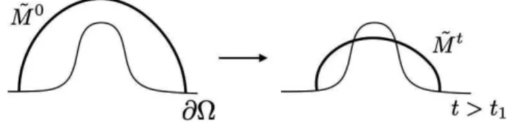
(5) 5. \partial\Omega t>t_{1} Figure 2: An example of the mean curvature flow with the right angle condition.. \Omega. Figure 3: A stationary solution to Brakke’s mean curvature flow with a generalized right angle condition such that \tilde{M}\cap\Omega consists of line segments.. boundary \partial\tilde{M} . If a family of smooth immersions F:\tilde{M}\cross[0, T ) flow. \{\tilde{M}^{t}\}=\{F(M, t)\} v_{M^{t}}-=h_{M^{t}}-. arrow \mathbb{R}^{n}. construct a geometric. such that. on. \tilde{M}^{t},. \partial\tilde{M}^{t}=F(\partial\tilde{M}, t)\subset\partial\Omega,. \nu_{M^{t} -\perp\partial\Omega. on. \partial\tilde{M}^{t},. where v_{M^{t}}- is the normal velocity vector of \tilde{M}^{t} , we say that \tilde{M}^{t} is a mean curvature flow with the right angle condition. Since F is a smooth map, \tilde{M}^{t} does not change the topology and it is possible that \tilde{M}^{t} moves to the outside \Omega . For example, in Figure 2, the moving hyper‐ surface \tilde{M}^{t} touch the boundary \partial\Omega at time t_{1}\in(0, T) and pass through it. From a physical point of view, we would like to construct a mean curvature flow “only inside \Omega ” by letting topological changes occur. Since topological changes are ones of the singularities, we study a weak solution to the mean curvature flow in the sense of Brakke. Here, we discuss the behavior of the Brakke’s mean curvature flow defined in Definition 2.3. If we assume that a Brakke’s mean curvature flow with a generalized right angle condition \mu^{t} is described as \mu^{t}=\mathcal{H}^{n-1}\lfloor M^{t}- for some smooth and orientable (n-1) ‐dimensional sub‐ manifold \tilde{M}^{t} in \mathbb{R}^{n} with compact and smooth boundary \partial\tilde{M}^{t} , we may see that for any t>0. (i) \tilde{M}^{t}\subset\overline{\Omega}, (ii) \partial\tilde{M}^{t}\subset\partial\Omega and. \nu_{M^{t}}-. is perpendicular to. \partial\Omega. on \partial\tilde{M}^{t},. (iii) v_{M^{t}}-=h_{M^{t}}- on \tilde{M}^{t}\cap\Omega. The property (i) follows from spt\mu^{t}\subset\overline{\Omega} and we do not know if \partial\Omega\cap\tilde{M}^{t}=\partial\tilde{M}^{t} . We also note that the definition of Brakke’s mean curvature flows with a generalized right angle condition do not tell us the behavior of \partial\Omega\cap\tilde{M}^{t} immediately. Indeed, \mathcal{H}^{n-1}\lfloor\partial\Omega and \mathcal{H}^{n-1}\lfloor_{M^{-} , where \tilde{M}\subset\overline{\Omega} is a hyper‐surface composed of a minimal surface \tilde{M}\cap\Omega and the remaining part.
(6) 6 \tilde{M}\cap\partial\Omega , are stationary solutions to the Brakke’s mean curvature flow with a generalized right. angle condition (see Figure 3). The motion of a measure \mathcal{H}^{n-1}\lfloor M^{t}- seems possible to converge. to the stationary solution \mathcal{H}^{n-1}\lfloor_{M^{-} in finite time, and in this case, \tilde{M}^{t} does not change the topology. Therefore, analysis on the behavior of the Brakke’s mean curvature flow with a generalized right angle condition, in particular construction of a motion with some topological changes, is a future work. We also note that, in broad strokes, the boundary condition of a level set formulation of the mean curvature flow with the right angle condition is defined by. \max\{\{\nu_{M_{a}^{t},M_{a}^{t}M_{a}^{t}}-\nu\}, v--h-\}\geq 0\geq\min\{\langle\nu_{M_{a}^{t},M_{a}^{t}M_{a}^{t}}-\nu\rangle, v--h-\} on the boundary. function. v. \partial\Omega. for any. : \Omega\cross[0, \infty ). arrow \mathbb{R} ,. a\in \mathbb{R} ,. where. \tilde{M}_{a}^{t}. is the level set. \{x\in\overline{\Omega} : v(x, t)=a\}. for a. in the viscosity sense (see [2, 3, 6, 9, 12] for more details).. Because of the boundary condition, the behavior of the level set flow is not well known. For. example, Giga [5] constructed a viscosity solution. v. in the case. n=2. so that the zero level set. of v(\cdot, t) fattens in finite time t_{0}>0 . By using this solution, we can construct two curvature flows with the right angle condition, which start frow same initial curve, so that one of the flows is separated into two curves for any t>t_{0} and the other does not change the topology.. 3 3.1. Assumptions and main result Assumptions of initial functions. Hereafter, we assume the following assumptions for the initial function u_{\varepsilon,0}\in C^{1}(\overline{\Omega}) of (1.1): (A1) \Vert u_{\varepsilon,0}\Vert_{L^{\infty}(\Omega)}\leq 1, (A2) there exists D_{0}>0 such that. \sup_{x\in\Omega,r>0}\int_{B_{r}(x)\cap\Omega}\frac{\varepsilon|\nabla u_{\varepsilon,0}(y)|^{2} {2}+\frac{W(u_{\varepsilon,0}(y) }{\varepsilon}dy\leq D_{0}r^{n-1},. (A3) there exists c_{1}>0 such that \sup_{x\in\Omega}\varepsilon|\nabla u_{\varepsilon,0}|\leq c_{1}, (A4) there exist c_{2}>0 and \lambda\in[3/5,1 ) such that (A5). \frac{\partial u_{\varepsilon,0} {\partial\nu}(x)=0. Here, let D_{0},. c_{1}, c_{2}. for. \sup_{x\in\Omega\frac{\varepsilon|\nabla u_{\varepsilon,0}(x)|^{2} {2} - \frac{W(u_{\varepsilon,0}(x) }{\varepsilon}\leq c_{2}\varepsilon^{-\lambda},. x\in\partial\Omega.. and \lambda\in[3/5,1 ) be some universal constants. By the standard parabolic. existence and regularity theory, for each. \varepsilon>0 ,. there exists a unique solution. u_{\varepsilon}\in C([0, \infty);C^{1}(\overline{\Omega}))\cap C^{\infty} (\overline{\Omega}\cross(0, \infty)) We also note that the boundedness of the domain. \Omega. u_{\varepsilon}. with. .. and the assumption (A2) imply. \sup_{i}E_{\varepsilon_{i} [u_{\varepsilon_{i},0}]\leq c_{3} for some constant. c_{3}. depending only on. n,. (3.1). D_{0} and the diameter of \Omega . Only the conditions. (A1), (3.1) and the regularity u_{0}\in H^{1}(\Omega) are assumed in [10]. Therefore, we note a choice of initial functions satisfying the assumptions (A1)-(A5) in the following remark..
(7) 7 Remark 3.1 We note that for a surface \Gamma with 90 degree contact angles on \partial\Omega it is possible to construct diffuse approximations that satisfy the assumptions (A1)-(A5) as the following.. Our construction is standard as in [7, 11]. Let \Omega_{d} be. \Omega_{d}:=\{(y_{1}, y')\in \mathbb{R}^{n}:y_{1}\in \mathbb{R}, |y'|<d\} for d>0 and define \tilde{\Gam a} :=\overline{\Omega}_{d}\cap\{y_{1}=0\} . By the standard existence theory for ordinary differential equations, we may choose the unique function q\in C^{4}(\mathbb{R}) such that. q(0)=0, sarrow\pm 1\dot{{\imath}}m_{\infty}q(s)=\pm 1, q'(s)=\sqrt{2W(q(s))} in \mathbb{R}. Then it is easy to see that the C^{4} function v_{\varepsilon_{i} (y) :=q(y_{1}/\varepsilon_{i}) defined on \overline{\Omega}_{d} satisfies. \int_{B_{r}(yo)\cap\Omega_{d} \frac{\varepsilon_{i}|\nablav_{\varepsilon_{i} |^{2} {2}+\frac{W(v_{\varepsilon_{i} ) {\varepsilon_{i} dy\leq\sigma\omega_{n-1} r^{n-1} \varepsilon_{i}|\nabla v_{\varepsilon_{i} (y)|\leq\max_{|s|\leq 1}\sqrt{2W(s)} , \langle\nabla v_{\varepsilon_{i} , \nu_{d}\rangle=0 where. \sigma. on. := \int_{-1}^{1}\sqrt{2W(s)}dx. Ũ is a neighborhood of. \tilde{r}. \phi (\Omega_{d}\cap\~{U}) =\Omega\cap U,. for r>0, y_{0}\in \mathbb{R}',. \frac{\varepsilon_{\dot{i}|\nablav_{\varepsilon_{\dot{i} (y)|^{2}{2}=\frac {W(v_{\varepsilon_{i}(y)}{\varepsilon_{\dot{i}. for y\in\overline{\Omega}_{d} ,. (3.2). \partial\Omega_{d},. and \nu_{d} is the out ward unit normal to. and that. \phi. \phi(\partial\Omega_{d}\cap \~{U}). \partial\Omega_{d} .. map from Ũ onto. Now we assume that. is a bijective. C^{1}. =\partial\Omega\cap U,. \sup_{x\in U}\Vert\nabla\phi^{-1}(x)\Vert\leq 1, \sup_{y\in\tilde{U} \Vert\nabla\phi(y)\Vert\leq C. U. : =\phi (Ũ) such that. for a suitable d>0 and a constant C>0 , where \Vert . \Vert is the operator norm. By using this. mapping, (3.2) implies that u_{\varepsilon_{i},0}(x) :=v_{\varepsilon_{i}}o\phi^{-1}(x) satisfies the assumptions (Al)-(A5) with. a positive constant D_{0} depending only on \sigma, n and C, c_{1}=1 and c_{2}=0 on the set \overline{\Omega}\cap U. By expanding u_{\varepsilon_{i},0} as a mostly constant function to satisfy the assumptions outside of U , we may see the possibility of the initial assumptions in the present paper. In this construction, the diffused interface energy for u_{\varepsilon_{i},0} should behave like the surface measure of the surface \Gamma :=\phi(\tilde{\Gamma}) and \Gamma intersects \partial\Omega with 9\theta degrees. 3.2. Main result. Our goal is to extend the convergence theory in [10] to remove the assumption of the convexity of the domain as the following.. Theorem 3.2 ([8]) Let \Omega\subset \mathbb{R}^{n} be a bounded domain with smooth boundary. Assume (A1)(A5) and let u_{\varepsilon} be the unique solution of (1.1) for \varepsilon>0 . Define a Radon measure \mu_{\varepsilon}^{t} by (1.2). Then, there exist a sub‐sequence \{\varepsilon_{i}\}_{i\in \mathb {N} converging to 0 as iarrow\infty and a set of Radon measures \mu^{t} on \mathbb{R}^{n} such that \mu_{\varepsilon_{i} ^{t}harpoonup\mu^{t}(iarrow\infty) in the sense of measure for all t\geq 0. Furthermore, \mu^{t} is a Brakke’s mean curvature flow with a generalized right angle condition defined by Definition 2.3.. Remark 3.3 The integrality of the limit Radon measures \mu^{t} in the interior of \Omega follows from. [16]..
(8) 8. \bullet.. \hat{\alpha}. \Omega. \zeta(*. ’. Figure 4: Picture of \zeta(x) and. 4. \tilde{x}.. Outline of proof. As we mentioned in Section 1, the equation (1.1) is a L^{2} ‐gradient flow of E_{\varepsilon} , therefore we obtain the uniformly boundedness of E_{\varepsilon}[u_{\varepsilon}(\cdot, t)] with respect to t>0 and \varepsilon>0 by applying (3.1). Roughly speaking, this fact and the compactness of Radon measure imply the conver‐ gence \mu_{\varepsilon_{i} ^{t}harpoonup\mu^{t}(iarrow\infty) . Here, we discuss the rectifiability of \mu^{t} (i.e. the condition (V1)).. We note that the condition spt\mu\subset\overline{\Omega} obviously follows from the convergence \mu_{\varepsilon_{i} ^{t}harpo nup\mu^{t} and the inclusion spt\mu_{\varepsilon}^{t}\subset\overline{\Omega} for any \varepsilon>0. One of the key arguments to prove the rectifiability of \mu^{t} is a characterization by the (n-1) ‐dimensional backward heart kernel. For y\in \mathbb{R}^{n} and s>0 , let \rho(y,s) be the (n-1)dimensional backward hear kernel, namely,. \rho_{(y,s)}(x, t). := \frac{1}{(4\pi(s-t) ^{\frac{n-1}{2} e^{-\frac{|x-y|^{2} {4(s-t)}. for. x\in \mathbb{R}^{n},. t<s .. (4.1). Roughly speaking, the heart kernel \rho_{(y,s)}(\cdot, t) converges to (n-1) ‐dimensional delta function on (n-1) ‐dimensional hyper‐surface as tarrow s in the sense of distribution. For example, if M is a smooth k ‐dimensional sub‐manifold in \mathbb{R}^{n} such that y is a interior point of M , then. 1t\dot{\imath}\uparowms\int_{M}\rho_{(y,s)}(x,t)d\mathcal{H}^{k}(x)= \{ begin{ar y}{l 0 ifk=n, 1 ifk=n-1, \infty ifk\leqn-2. \end{ar y}. Therefore, the “dimension” of \mu^{t} can be analyzed by \mu^{t}(\rho_{(y,s)}(\cdot, t)) and this analysis is a first step to prove the rectifiablity of \mu^{t} . The Huisken or Ilmanen type monotonicity formula is an inequality to control the time development of \mu^{t}(\rho_{(y,s)}(\cdot, t)) , thus we define some notions to present the statement of the monotonicity formula. The following notions are related to the reflection argument. Define \kappa as \kappa. For. s>0 ,. :=\Vert principal curvature of \partial\Omega\Vert_{L^{\infty}(\partial\Omega)}.. define a subset N_{s} of. \mathbb{R}^{n}. by. N_{s} :=\{x\in \mathbb{R}^{n}:dist(x, \partial\Omega)<s\}..
(9) 9 There exists a sufficiently small. c_{4}\in(0, (6\kappa)^{-1}]. depending only on \partial\Omega such that all points x\in N_{6c_{4}} have a unique point \zeta(x)\in\partial\Omega such that. dist (x, \partial\Omega)=|x-\zeta(x)| (see also Figure 4). By using this \zeta(x) , we define the reflection point \tilde{x}. of. x. with respect to \partial\Omega as. \tilde{x}:=2\zeta(x)-x. We also fix a function. \eta\in C^{\infty}(\mathbb{R}). \frac{d\eta}{dr}\leq 0,. 0\leq\eta\leq 1, For. s>t>0. and. x,. such that. spt\eta\subset[0, c_{4}/2) ,. \eta=1. on. [0, c_{4}/4].. y\in N_{c_{4}} , we define the truncated version of the (n-1) ‐dimensional. backward heat kernel and the reflected backward heat kernel as. \rho_{1,(y,s)}(x, t) :=\eta(|x-y|)\rho_{(y,s)}(x, t) , \rho_{2,(y,s)}(x, t) := \eta(|\tilde{x}-y|)\rho_{(y,s)}(\tilde{x}, t). ,. where \rho_{(y,s)} is defined as in (4.1). For x\in N_{2c_{4}}\backslash N_{c_{4}} and y\in N_{c/2}4 , we have. | \tilde{x}-y|\geq|\tilde{x}-\zeta(y)|-|\zeta(y)-y|>c_{4}-\frac{c_{4} {2}=\frac {c_{4} {2}. Thus we may smoothly define \rho_{2,(y,s)}=0 for x\in \mathbb{R}^{n}\backslash N_{c4} and y\in N_{c_{4}/2} . We also define the discrepancy function \xi_{\varepsilon_{i} as. \xi_{\varepsilon_{i} (x, t). := \frac{\varepsilon_{i}|\nabla u_{\varepsilon_{i} (x,t)|^{2} {2}- \frac{W(u_{\varepsilon_{i} (x,t) }{\varepsilon_{i}. for. (x, t)\in\overline{\Omega}\cross[0, \infty ).. Proposition 4.1 (Boundary monotonicity formula [10]) There exist constants 0<c_{5}, \infty. depending only on. n, c_{3}. c_{6}<. and \partial\Omega such that. \frac{d}{dt}(\sigma e^{c_{5}(s-t)z}1\int_{\Omega}\rho_{1,(y,s)}(x, t)+\rho_{2, (y,s)}(x, t)d\mu_{\varepsilon^{i} ^{t}(x) \leq e^{c_{5}(s-t)^{\frac{1}{4} }(c_{6}+\int_{\Omega}\frac{\rho_{1,(y,s)}(x,t) +\rho_{2,(y,s)}(x,t)}{2(s-t)}\xi_{\varepsilon_{i} (x, t)dx). (4.2). for all s>t>0, y\in N_{c4/2} and i\in \mathbb{N},. \frac{d}{dt}(\sigma e^{c_{5}(s-t)^{\frac{1}{4} \int_{\Omega}\rho_{1,(y,s)}(x, t)d\mu_{\varepsilon^{i} ^{t}(x) \leq e^{c_{5}(s-t)^{\frac{1}{4} (c_{6}+ \int_{\Omega}\frac{\rho_{1,(y,s)}(x,t)}{2(s-t)}\xi_{\varepsilon_{i} (x, t)dx) for all s>t>0, y\in \mathbb{R}^{n}\backslash N_{c/2}4 and. i\in \mathbb{N} ,. where. \sigma. (4.3). is the constant defined by (1.3).. The proof of Proposition 4.1 in [10] does not require the convexity of. \Omega ,. thus we can. apply this monotonicity formula to our problem. In order to control the time evolution of \mu^{t}(\rho_{(y,s)}(\cdot, t))(\approx\mu^{t}(\rho_{1,(y,s)}(\cdot, t)+ \rho_{2,(y,s)}(\cdot, t))) , we have to take the limit iarrow\infty for both. inequalities (4.2) and (4.3). Therefore, analysis on the behavior of the discrepancy function \xi_{\varepsilon_{i} with respect to i is one of the key arguments. In the following, we study the upper bound of the discrepancy function..
(10) 10 4.1. Preparation. In this section, we note some lemmas to discuss estimates on the upper bound of the discrep‐ ancy function. A key lemma is the following equality to control the normal derivative of the discrepancy function.. Lemma 4.2 Let A_{x} be the second fundamental form of. \frac{\partial}{\partial\nu}\frac{|\nablau_{\varepsilon_{i} |^{2} {2}=A_{x} (\nablau_{\varepsilon_{i} ,\nablau_{\varepsilon_{i} ). for. \partial\Omega. at x\in\partial\Omega . Then. (x, t)\in\partial\Omega\cross(0, \infty) .. This equality can be proved by using only the Neumann boundary condition of (1.1). We also note that Lemma 4.2 and the Neumann boundary condition of (1.1) imply that for any (x, t)\in\partial\Omega\cross(0, \infty). \frac{\partial}{\partial\nu}\xi_{\varepsilon_{i}\leq\{ begin{ar ay}{l} 0 if\Omegaisconvex, \kap ae_{i}|\nablau_{i}|^{2} ev nif\Omegaisnotconvex. \end{ar ay}. (4.4). Another key lemma is an estimate which follows from the scaling argument. Let. \Omega_{\varepsilon_{i} =\{y\in \mathbb{R}^{n}:\varepsilon_{i}y\in\Omega\} and define the function. v_{\varepsilon_{i} (y, \tau) :=u_{\varepsilon_{i} (\varepsilon_{i}y, \varepsilon_{i}^{2}\tau). for. y\in\overline{\Omega}_{\varepsilon_{i} ,. \tau\in[0, \infty ).. We note that. \kap a_{\varepsilon_{i}. :=|lprincipal curvature of. (4.5). \partial\Omega_{\varepsilon_{i} \Vert_{L\infty(\partial\Omega_{\varepsilon_{i} )}=\varepsilon_{i}\kap a. holds and v_{\varepsilon_{i} satisfies. \{begin{ar y}{l \partil_{\tau}v_{\arepsilon_{i}=\trianglev_{\arepsilon_{i}- W'(v_{\arepsilon_{i})n\Omega_{\varepsilon_{i}\cros(0,\infty), \{nabl v_{\arepsilon_{i},\nu_{\varepsilon_{i}\=0on \partil\Omega_{\varepsilon_{i}\cros(0,\infty), \end{ar y} where \nu_{\varepsilon_{i} is the outward unit normal to \partial\Omega_{\varepsilon_{i} . The standard gradient estimate depends on the second fundamental form of the boundary of the domain. Therefore, “uniformly gradient. estimate” of v_{\varepsilon_{i} holds by (4.5), namely, |\nabla v_{\varepsilon_{i} | is uniformly bounded with respect to if. \sup.\in\overline{\Omega}_{i},i\in \mathbb{N}|\nabla v_{\varepsilon_{i} (x, 0) |. and. \varepsilon_{i}. is finite. Since the boundedness of \nabla v_{\varepsilon_{i} at initial time is equivalent. to the assumption (A3), we obtain the following estimate. Lemma 4.3 There exists a constant. c_{7}. depending only on. \sup \varepsilon_{i}|\nabla u_{\varepsilon_{i} |\leq c_{7}. \Omega\cross[0,\infty). for all 0<\varepsilon_{i}<1.. x, t. c_{1}, c_{4}. and. W. such that.
(11) 11 11. Remark 4.4 By the scaling argument, we can obtain the uniformly boundedness of the second derivatives of v_{\varepsilon_{i} if we assume the uniformly boundedness of its derivatives at initial time. Therefore, roughly speaking, the estimate |\nabla^{2}u_{\varepsilon_{i} |\les approx\varepsilon_{i}^{-2} follows from the scaling argument under suitable assumptions, which gives the estimate |\langle\nabla\xi_{\varepsilon_{i} , \nu\rangle|\les ap rox\varepsilon_{i}^{-2} On the other hand,. by combining (4.4) and Lemma 4.3, we obtain. \frac{\partial}{\partial\nu}\xi_{\varepsilon_{i}\leq\kap ac_{7}^{2} \varepsilon_{i}^{-1}. (x, t)\in\partial\Omega\cross[0, \infty ). for. (4.6). which is better than the estimate following from the scaling argument in the viewpoint of the oder of \varepsilon_{i}. We also note that the estimate \xi_{\varepsilon_{i} \les ap rox\varepsilon_{i}^{-1} can be obtained by Lemma 4.3 since \sup.,t|u_{\varepsilon_{i}}|\leq 1. follows from the maximum principle and the assumption (Al). Our aim is to obtain a better. estimate of the upper bound of the discrepancy function in the viewpoint of the oder of. 4.2. \varepsilon_{i}.. Upper bound of discrepancy function on CONVEX domains. First, we discuss the upper bound of discrepancy in the case that. \Omega. is convex. By the Allen‐. Cahn equation (1.1) and a simple calculation, we obtain. \parti l_{t}\xi_{\varepsilon_{i}-\triangle\xi_{\varepsilon_{i}\leq- \frac{2\langleW'(u_{\varepsilon_{\dot{i} )\nabl u_{\varepsilon_{i}, \nabl \xi_{\varepsilon_{i}\rangle}{\varepsilon_{i}^2}|\nabl u_{\varepsilon_{i}'|^{2}. on. \{(x, t)\in\Omega\cross(0, \infty) : |Vu_{i}|\neq 0\} .. (4.7). Here, we have used the Cauchy‐Schwarz inequality. |\nabla^{2}u_{i}|^{2}|\nabla u_{\varepsilon_{i} |^{2}\geq|\nabla^{2} u_{\varepsilon_{i} \nabla u_{\varepsilon_{i} |^{2}. We note that \xi_{\varepsilon_{i} is obviously non‐positive if |\nabla u_{\varepsilon_{i}}|=0 .. Therefore, if. \Omega. is convex, the. maximum principle for the discrepancy function works well by virtue of (4.4) and (4.7), and Mizuno and Tonegawa [10] proved the uniformly boundedness \xi_{\varepsilon_{i} \leq C for some C>0 being independent of. 4.3. x, t. and. \varepsilon_{i}. via this argument.. Upper bound of discrepancy function on NON‐CONVEX domains. Our aim is to extend the convergence theory in [10] to remove the assumption of the convexity of the domain. Therefore, we estimate the upper bound of the discrepancy function without the assumption of the convexity of the domain as the following. Proposition 4.5 There exists a constant. c_{8}. n, \kappa, c_{1}, c_{2}, c_{4}, W. depending only on. and. \Omega. such. that. \sup\frac{\varepsilon_{i}|\nablau_{\varepsilon_{\dot{i} |^{2}{2}- \frac{W(u_{\varepsilon_{i}){\varepsilon_{i}\leqc_{8}\varepsilon_{i}^{- \lambda}. (4.8). \Omega\cross[0,\infty). for any 0<\varepsilon_{i}<1 , where. \lambda. is the constant in the assumption (A4).. In the following, we assume 3/5<\lambda<1 for simplicity. We define a function based on the distance function dist (\partial\Omega, \cdot) from \partial\Omega by. \phi_{\varepsilon_{i} (x) :=\kappa(c_{7}^{2}+1)\psi(dist(\partial\Omega, x) /\varepsilon_{i}). ,. \phi_{\varepsilon_{i} \in C^{\infty}(\overline{\Omega}).
(12) 12 where. \psi\in C^{\infty}([0, \infty);\mathbb{R}^{+}) \psi(s)=s. satisfies. for s\in[0, c_{4}/2],. \psi'(s)=0. |\psi'|\leq 1,. for s\in[c_{4}, \infty ),. |\psi"|\leq 4/c_{4}.. By applying the standard estimates of the derivatives of the distance function dist (\partial\Omega, \cdot) , we obtain. \frac{\partial}{\partial\nu}\phi_{\varepsilon_{i}=-\frac{\kap a(c_{7}^{2}+1)} {\varepsilon_{i}. on. (4.9). \partial\Omega. and. 0<\phi_{\varepsilon_{i}}\leq M_{1},. \triangle\phi_{\varepsilon_{i} \leq M_{1}/\varepsilon_{i}^{2} in. |\nabla\phi_{\varepsilon_{i} |\leq M_{1}/\varepsilon_{i},. \Omega. (4.10). n, \kappa, c_{4} and c_{7} . Define G\in C^{\infty}(\mathbb{R}) by is the constant in the assumption (W2). We note that G(u_{\varepsilon_{i} ). for some positive constant M_{1} depending only on. G(s) :=1-(s-\gamma)^{2}/S , where. \gamma. satisfies. 0<G(u_{\varepsilon_{i} )<1, G'(u_{\varepsilon_{i} )W'(u_{\varepsilon_{i} ) \geq 0, G"(u_{\varepsilon_{i} )=-\frac{1}{4} . Let. \tilde{\xi}_{\varepsilon_{i}. (4.11). is a modified discrepancy function defined by. \tilde{\xi}_{\varepsilon_{i} (x, t) :=\xi_{\varepsilon_{i} (x, t)-\varepsilon_{ \dot{i} ^{-\lambda}G(u_{\varepsilon_{i} )+\phi_{\varepsilon_{i} (x). .. Then, by virtue of (4.10) and (4.11), we may see the equivalence. \xi_{i}\les approx e_{i}^{-\lambda}. in. \Omega\cros [0, \infty)\Leftrightar ow\tilde{\xi}_{\varepsilon_{i} \les approx\varepsilon_{i}^{-\lambda}. \Omega\cross[0, \infty) .. in. Therefore, it is sufficient to prove the estimate on the left hand side of the equivalence. By a. similar argument for (4.7), we obtain. \partial_{t}\ilde{\xi}_{\varepsilon_{i}-\triangle\tilde{\xi} _{\varepsilon_{i}\leq-\frac{2\{ nabla\tilde{\xi}_{\varepsilon\prime} l(W'(u_{\varepsilon_{i}\prime)+\varepsilon_{i}^{1-\lambda}G'(u_{\varepsilon_{i} \prime)\nablau_{\varepsilon_{\dot{i} -\nabla\phi\}{\varepsilon_{\dot{i} ^{2}|\nablau_{\varepsilon_{\dot{i} |^{2}-\varepsilon_{i}^{-\lambda-2} G'(u_{\varepsilon_{i})W'(u_{\varepsilon_{i}) +\varepsilon_{i}^{-\lambda}G"(u_{\varepsilon_{i})|\nablau_{\varepsilon_{i} |^{2}+\frac{2(W'(u_{\varepsilon_{i})+\varepsilon_{i}^{1-\lambda} G'(u_{\varepsilon_{i}.)}{\varepsilon_{i}^{2}|\nablau_{\varepsilon_{i}.|^{2} \{ nablau_{\varepsilon_{i},\nabla\phi\}+\triangle\phi on. \{(x, t)\in\Omega\cross(0, \infty) : |\nabla u_{\varepsilon_{i}}|\neq 0\}.. By applying the inequalities (4.10) and (4.11), it implies. \partial_{t}\ilde{\xi}_{\varepsilon_{i}-\triangle\tilde{\xi} _{\varepsilon_{i}\leq-\frac{2\{ nabl \tilde{\xi}_{\varepsilon_{\dot{x} ,(W'u_ {\varepsilon_{\dot{i} )+\varepsilon_{i}^1-\lambda}G'(u_{\varepsilon_{\dot{i} )\nabl u_{\varepsilon_{i}-\nabl \phi\rangle}{\varepsilon_{i}^2}|\nabl u_{\varepsilon_{\dot{i} |^{2} +\frac{M_{2} \varepsilon_{\dot{i}^{3}|\nabl u_{\varepsilon_{\dot{i} |- \frac{\varepsilon_{i}^-\lambda}{4|\nabl u_{\varepsilon_{i}|^{2}+\frac{M_{1} {\varepsilon_{i}^2} on. \{(x, t)\in\Omega\cross(0, \infty):|\nabla u_{\varepsilon_{i}}|\neq 0\},. where M_{2} is a positive constant depending only on M_{1} and. hand, (4.6) and (4.9) imply. \frac{\partial}{\partial\nu}\tilde{\xi}_{\varepsilon_{i}<0. on. \partial\Omega\cross(0, \infty) .. (4.12). \sup_{|s|\leq 1}|W'(s)| . On the other.
(13) 13 Therefore, we can apply a modified maximum principle for the modified discrepancy function. Indeed, if we assume. \tilde{\xi}_{\varepsilon_{i} (y, \tau)= \sup \tilde{\xi}_{\varepsilon_{i} (x, t)=C\varepsilon_{i}^{-\lambda} (x,t)\in\Omega\cross(0,T). for sufficiently large C>0 and a fixed time at the point (y, \tau) shows. T>0 ,. then. y. is a interior point of. \Omega. and (4.12). 0\leq\tilde{C}_{1}(\varepsilon^{\frac{\lambda-5}{i^{2} +\varepsilon_{i}^{-2})- \tilde{C}_{2}\varepsilon_{i}^{-1-2\lambda},. where the constants \tilde{C}_{1} and \tilde{C}_{2} are positive and independent of \varepsilon_{i} and T>0 . However this is a contradiction for sufficiently large i\in \mathbb{N} because the right hand side diverges to -\infty as iarrow\infty . Therefore, we have the conclusion.. Remark 4.6 Roughly speaking, Lemma 4.2 and (4.7) give improved estimates for the order of \varepsilon_{i} , which are better than the estimates following from the scaling argument (see Remark 4.4). The inequality (4.8) corresponds to one kind of “interpolation inequality” between the inequalities (4.6) and (4.7), thus the fractional exponent \lambda appears in (4.8). 4.4. Vanishing of the discrepancy. By applying the inequality (4.8), we can prove. \int_{t_{1} ^{t_{21} e^{c_{5}(s-t)^{z} \int_{\Omega}\frac{\rho_{1,(y,s)}(x,t)+ \rho_{2,(y,s)}(x,t)}{2(s-t)}\xi_{\varepsilon_{i} (x, t)dxdtar ow 0. as. iarrow\infty. for 0\leq t_{1}<t_{2}\leq s . Therefore, we can take the limit iarrow\infty for (4.2). The proof is based on the argument by [15]. Here, we note that we have to modify the argument to include the reflection argument.. References. [1] W. K. Allard, On the first variation of a varifold, Ann. of Math. 95 (1972), pp417‐491. [2] G. Barles and F. Da Lio, A geometrical approach to front propagation problems in bounded domains with Neumann‐type boundary conditions, Interface Free Bound. 5 (2003), pp239‐ 274.. [3] G. Barles and P. E. Souganidis, A new approach to front propagation problems: theory and applications, Arch. Rational Mech. Anal. 141 (1998), pp237‐296. [4] L. C. Evans and R. F. Gariepy, Measure theory and fine properties of functions, Studies in Advanced Math., CRC Press, Revised ed., (2015). [5] Y. Giga, Evolving curves with boundary conditions, Curvature flows and related topics, GAKUTO Internat. Ser. Math. Sci. Appl. 5 (1995), pp99‐109. [6] Y. Giga and M.‐H. Sato, Neumann problem for singular degenerate parabolic equations, Differential Integral Equations 6 (1993), pp1217‐1230..
(14) 14 [7] T. Ilmanen, Convergence of the Allen‐Cahn equation to Brakke’s motion by mean curva‐ ture, J. Diff. Geom. 38 (1993), pp417‐461. [8] T. Kagaya, Convergence of the Allen‐Cahn equation with a zero Neumann boundary con‐ dition on non‐convex domains, accepted to appear in Math. Ann. https://rdcu.be/2zf2 [9] M. Katsoulakis, G. T. Kossioris and F. Reitich, Generalized motion by mean curvature with Neumann conditions and the Allen‐Cahn model for phase transitions, J. Geom. Anal.. 5 (1995), pp255‐279. [10] M. Mizuno and Y. Tonegawa, Convergence of the Allen‐Cahn equation with Neumann boundary conditions, SIAM J. Math. Anal. 47 (2015), pp1906‐1932. [11] L. Modica, The gradient theory of phase transitions and the minimal interface criterion, Arch. Rational Mech. Anal. 98 (1987), pp123‐142. [12] M.‐H. Sato, Interface evolution with Neumann boundary condition, Adv. Math. Sci. Appl. 4 (1994), pp249‐264.. [13] L. Simon, Lectures on geometric measure theory, Proceedings of the Centre for Mathe‐ matical Analysis, Australian National University 3 (1983). [14] A. Stahl, Regularity estimates for solutions to the mean curvature flow with a Neumann boundary condition, Calc. Var. Partial Differential Equations 4 (1996), no. 4, pp385‐407. [15] K. Takasao and Y. Tonegawa, Existence and regularity of mean curvature flow with trans‐ port term in higher dimensions, Math. Ann. 364 (2016), no. 3‐4, pp857‐935.. [16] Y. Tonegawa, Integrality of varifolds in the singular limit of reaction‐diffusion equations, Hiroshima Math. J. 33 (2003), pp323‐341. Institute of Mathematics for Industry Kyushu University Fukuoka 819‐0395. JAPAN. E‐mail address: [email protected]‐u.ac.jp.
(15)
図


関連したドキュメント
Bouziani, Rothe method for a mixed problem with an integral condition for the two-dimensional diffusion equation, Abstr.. Pao, Dynamics of reaction-diffusion equations with
[7] , On initial boundary value problem with Dirichlet integral conditions for a hyperbolic equation with the Bessel operator, J.. Bouziani
Cannon studied a problem for a heat equation, and in most papers, devoted to nonlocal problems, parabolic and elliptic equations were studied.. Mixed problems with nonlocal
For arbitrary 1 < p < ∞ , but again in the starlike case, we obtain a global convergence proof for a particular analytical trial free boundary method for the
The goal is to prove the existence and uniqueness of a weak solution to the problem in the case when the nonlinearity in the Newton boundary condition does not satisfy any
Solov’ev, On an integral equation for the Dirichlet problem in a plane domain with cusps on the boundary..
Kiguradze, On some singular boundary value problems for nonlinear second order ordinary differential equations.. Kiguradze, On a singular multi-point boundary
The first paper, devoted to second order partial differential equations with nonlocal integral conditions goes back to Cannon [4].This type of boundary value problems with
