Estimation of the Rainfall Energy Affecting on the Ｇround

(1)

Estimation

of the Rainfall Energy

Affecting on the Ｇrｏｕnd･

NOBUHIRO MINAMI and Masazumi OGURA

ＬａｂｏｒａtｏｒｙｏｆＬａｎｄＣｏｎｓｅｒｖａｔｉｏｎ, ＦａｃｕltｙｃがＡｇｒicｕｌｔｕｒｅ

Abstract : Many investigations on the terminal velocity of ａ,rain drop and the distribu-tion of raindrops with their diameters in a storm, are totally concerned in rainfall energy･ We proposed semi theoretical equations of rainfall energy refering above investigations and introducing the relationship that count of raindrops per unit area and unit time are shown in the function of rainfall intensity･

These equations are compared with the others rainfall energy.equations in Fig. 6. This paper is described as the basic research for the study of soil erosion by rainfall.

Introduction

The first stage in the process of soil erosion by a storm is in the splash erosion. In this stage, we will require the estimation of ａ rainfall energy to discuss on movement of soil particles.

Results of investigations on the terminal velocties of every raindrop diameters, drop size distribution in unit space have been published. Let us discuss above terms by turns.

Terminal velocity and mass of ａ raindrops

Terminal velocities of raindrops depending on their sizes are attained when the gravitatio-nal forces oh their drops are balanced the resistance forces of the air through which they are falling respectively.

Published reports by ＬａｗSI）and Gunn and Kinzer^) are representative on falling velocity of ａ raindrop. The former measured their velocities by camera and the latter done by electric charge method for oscillograph recorder. Their results of ｍｅａ‘surment are in good agreement.

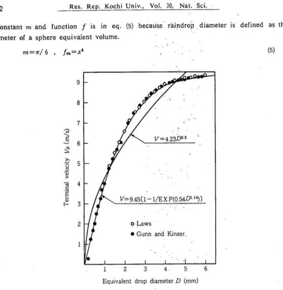
Terminal velocities of various size drops are plotted in Fig. 1 , where equivalent drop diameter is defined as the diameter of a sphere of equivalent volume.

Ａ general equation on the relationship between relative terminal velocity ｙ and veloctity function including drop size is expressed in eq. (l) Constants V and the function/, have been･

showed by Gunn and Ｋｉｎｚｅr2リｎeq. (2) simply. We will show them･１ｎeq. (3) closely. ｙ＝り1 （1）り= 4..23' 几＝jz7o●5 （2）ﾌ■>=9.45 石＝1 − 1 /EXP （0.54ｚ1.14）（3）丿 wherｅ￡）（ｍｍ）:equivalent diametｅｒ Do＝1（ｍｍ） ’ｙｚ，（ｍ/S）:terminal velocity ｙo＝1（ｍ/S）エ＝ＤノDo ﾌﾉ＝ら/ｙo .

Mass of ａ raindrop Mn (mg) is expressed generally in eq. (4)･

(2)

Constant

77z and function j is in eq. (5) because raindrop いdiameter is defined as the diameter of a sphere equivalent volume.

ｍ＝7ｒ/ 6 ，ふ＝ｚs ⊃ ノ▽ ● （5）９８７ < ￡ ) i n -^ ＣＯ︵Ｓ／ U I ) Ｏｙ＼ＡｊｐＯｌＳＡ J ＢＵ I ＵＵ９ＪＬ２１１２３４一一 5 6 Equivalentdrop diameter D (mm)

Fig. 1. Terminal velocity of water･drops･ of defferent ･sizes in a stagnant air and representative curve by equatio瓦j へ

Count and amount distribution of ｒ４血drops in unit space

We consider that in ａ continuous rainfall with constant iポensity, raindrops belong to in several classes of the range from (￡)−j￡)/2)t6▽(￡)ナｄＤ/1). which have representative diameter Ｄ respectively, and the origin of time 励d been defined the just time when ａ marking raindrop in each classes had landed ｏｎ'the ground surface.

After the time pass in dt, those Ｎぶh raindrops 'jn ･each classes (￡)土j￡)/2) have been landed on the ground which is in unit area Ｓ. " 犬 ‘ ・

It seems that at the origin of time Z＝O those iVnthかｏ恥y had eχisted upward from the ground surface in the space with the height of Ydt and raindrop flecks ofｙ counts have been made one after another by raindrops of Ｎ counts in the space･

According to this consideration, count density of raindrops in the space ｙoｚ,(ｍ-３ｍｍ-1) is expressed in eq. (6) physically and eq. (7) mathematically｡

(3)

e ａＳ r ５ａａ

㈲

1ろＮＱ。＝ａＮｏｆｏｆｏ＝＼/ＥχＰ（か/λ）〔7〕 where αｊ : constant, 7Vo＝1（７ｎ-> ｍｍ ^） λ:distribution factor

ゐ＝1 by Marshall and Parmer" ゐ＝2 by Shiotsuki'"

lf瓦。is defined in eq. (8), total count of raindrops ｊＶＪ（ｍ-3）ａｎｄthe probable count density function of raindrops /,, in the space are shown in eq. (9) and (1()。

F<Sn ゜Ｊｏ几血 (8)

ＮＪ＝f77ｖon ｄＬ)＝ｙoDOFo,i (9)

偏＝No。￡),/ＮＪ＝石/Fo。ぐ1(1

iS

二二で7でj≒yhith弛Ｄ土dDIl of the di“｢Tieterrange in the space Ｍｏ°(｢Tig/ ｢゜“1｣

Ｍ。＝ＭｂＮｏＤ＝ＰＪ＾oZ:)o3mムダo 圓

de

lごここjjﾀｯﾌﾟなｅご

｡

(1‰t:ｺﾞごSs of moisture Aも(tng/ ｢) and the probable moisture

Ｆ如、＝Ｊ°゜み几心; ０ＭＪ＝ f°゜肩 oJ￡)＝pjｖｏＤｏ’ ■ｍａＦｎ、 0 几。= -W0J9￡)/ＭＪ＝ふ几/Fo。

Count of raindrop flecks on the ground and ｒai皿fall intensity

If it is defined thａｌＮｏＤ{＼lmm ｢s).is count of raindrop flecks on the unit area of ground during unit time in the range Ｚﾆ)±ｄＤ/2 0f the raindrop size, we obtain eq. tt5).

Ｎｏ。＝Ｎ。Ｚ(ＳｄはL))＝Noｚ,ら＝ｙo7Voり可Jo 回 If F, is defined in eq. (16),total count of raindrop flecks Ｎ(1/m2S)ａｎｄ probable count density function of them are shown as eq.(17) and C18)｡

几＝j｀゜O 几石血旧

iV=Fcμoz:)四几聞ｆヶ，＝ＮｏｕI-:)/Ｎ＝ｆＪｏ/几 m

Total volume of raindrops landed during unit time‘on the unit area ･of ground means rainfall intensity /(mmV ｢s), therefore amount density of rainfall ら(ｍｍ２/m2S)iS shown in eｑバ19)｡乙＝ＭｄＮｑｄ/Ｐ。=VoNoL:)0^ｍｖafmfJo 叫

If Ft is defined in eq. (20)rainfall intensity ７ and probable amount density function 五 are shown as eq. 闇and (22)｡

(4)

J

0ﾍﾟ添)血

７＝Ｌ

/<=/^f,ふ/Ｆ。

Hence, from eq. iXD and (21], eq. (23) will be born.

I/NDo3＝琲Ｆ,/Ｆｎ

I 闘

(22)

(23)

If /o=(mm/h)

and Ｎａ＝＼（1/ｍｍh) are defined, / and

N

are measured

by those units

non dimensional numbers

as eq. (24)are producted.

i ＝ I/Io 、71＝Ｎ/Ｎｏ

Eq. (24) is rewriten as eq. (25). 百加＝ｍＦも/Ｆｎ

(24)

闇

If observed values of (φT.} are shown in the ･function e-(0, which have only one variable (０，･ｅｑ.･(25)is exchanged to ｅqバ26) which will show the relationship between ｆ and λ.

g（０＝ｍＦ４/Ｆ。＝人λ）

闘

Rainfall energy

li Ｅｌ,’（10-6J/ ｢mm)is defined as the rainfall energy affecting on the unit area of ground in each raindrop size range （￡）±dDIl) during unit time, it is as eq. 飢

￡ｙ＝Ｍｚ,ｙｊｙ２,/2===pt。Fo'NoDo’ｍｉｊ'af＾fjo (27)

When the rainfall energy per unit area and unit rainfall intensity is defined as ￡o instead of eq. 囲．

￡．＝EjZI＝（らｙo2/2Do）ｖＨｒ．fJo/瓦雛 If F， is defined as eq. (29), total energy E (J/m'mm) affecting on the unit area of ground

per unit rainfall intensity and probable density function of the energy /≪ are shown as eq. 閤and (3D. ダ．

F。＝J゛フムLhdx

￡＝fy￡Ｊ￡)＝￡002/2)瓦/几

石＝ふ几3几/Ｆ，

Where Ｅ,＝ρぶ

Definite

integral values

In this paper. four kinds of basic functions have been used as Table l

S５

^

ＥＪ

２２

(5)

15

1.0 2.0

Tabχｅ: V. Ｃｏｍｂｉｎａtｉｏｎｏｆｂａｓｉｃｆｕｎｃｔｉｏｎｓ

combination function is defined as （j､k）

Definite integral values of combination

functions in. two cases「1」)

and (1｡2)

can; be

obtained in Gamma

function with parameter

λas in Table 2.

In the other cases (2.1) and (2.2), those

values were obtained by Newton

･Cotes.･nu-merical inte!grationmethod

with several λ.

Relationship between those values and λ

is shown in Fig. 2.

5.0 1.0 ︱ｇｎｆＥＡ [ Ｂｉｓ a i ｕ i J i ｕ i j ｓｎ Table ｌ，ＶａｌｕｅｓｏｆＦ。，Ｅt，ａｎｄＦ６．ノ／〆 (2.1) ／ｇ／

づ

／／／／／／／／／／ _／

／

／／

／

１ノ／

ド

ｐ

／／／／／／／／

／

_／

／

//

／ｆ／ｊ／／／／／／ 0.003 1- 0.1 5.0 1.0 0.1 0.01 (2.2) ｜／／

／／

／

ｙ／がン

／

／／／／／ｒノ −／、／ , ノ？／ノ／

／

／ｙ

ル

ダ

／

ｒ／／／／／／ r 0 0 00？i λ Å Fig. 2. Definite in:tegral ｖａ]ues and λ.

(6)

2 0 ₂₅

Results of observation and discussion

Equivalent diameter of ａ raindrop Members in the Laboratory of Agricultural Meteoro-logy of Kyushu University have used the calibrattion curve t｀ｏ estimate the equivalent diameter from ａ fleck diameter Ｄ／ of ａ raindrop landed on the filter paper soaked Methylene Blue. ゛

This calibration curve is expressed in eq. (32).

x=0.305(Z:)ｒ/Do)゜●78 ¨ (32)

Observation data We counted raindrop flecks on the filterpaper in 18cm X 20cm area. This paper had been offered from Kyushu University and we calculated equvalent diameters by eq. (32》.Data are in Table ３｡

Tab＼e 3. Obｓｅｒｖａtｉｏｎｄａta i,1 1９８1

no.

date

exposed

time 7

(S)

count of drops

_{intensity of rain}

iヲ(π/6)Σ￡)5N≪dD/Io

i/n

y (1/360cm2Ts)

n=N/N。

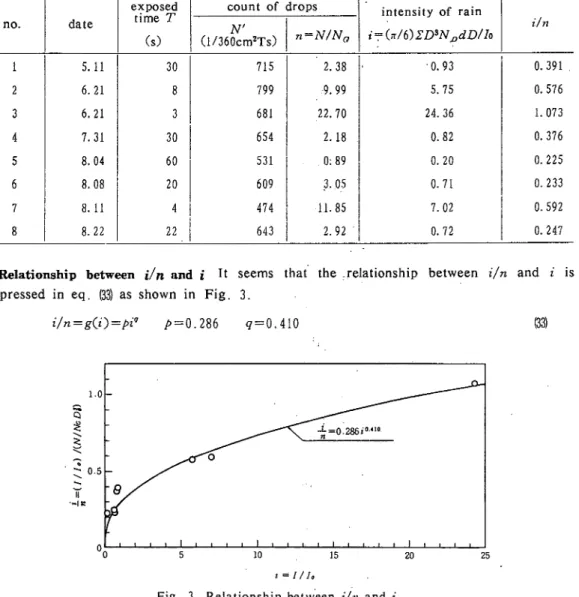
１２３４５６７８ 5.11 6.21 6.21 7.31 8.04 8.08 8.11 8.22 30 8 3 30 60 20 4 22 715 799 681 654 531 609 474 643 2.38 ,･9.99 22. 70 2.18 0:89 3.05 ↓1.85 2.92 1 ，･0.93 5.75 24.36 0.82 0.20 0.71 7.02 0､n 0.391 ， 0.576 1.073 0.376 0.225 0.233 0.592 0.247

Relationship between i/n and i It seems that the relationship between φz and i is expressed in eq. （3l as shown in Fig. 3.

φz＝ｇ（０＝μ９ i!> = 0.286 9 = 0.410 (33) ︵ｔａ＾Ｎ／Ｎ︶／ ( ≫ ／／／ ) = ？ 1.0 0.5 ００ 5 10 15 t＝□1。

(7)

邨; t;￨≪> ヽ卜 1 0 １０．１ 17

The relationship will suggest that average volume of ａ drop increase proportionally to the 9 th power of rainfall intensity.

Therefore in cases (1.1) and (1.2) values of ＼ are obtained from eq. (34)and 05). λ＝〔(6/π)(ｒ,.Ｊｒ４.5)が9ｙ3 闘 λ＝〔(6A)Cro.75/r2.25>!゜〕2/3 (35) In the other cases (2.1) and (2.2) values of λare obtained graphycally in Fig. 4.

-(2.1)-｜１

ぷ

／｜

聊

_九

才

ｙ

/

ノ〆〆 50 20 10 司絢５２ / / ｜〆

研

／〃ノｆ

/

ｆ ’ ／ _１ /￣￣ｆ ’

／

ｊ₋／「 − _-4

ル

／

Ｚｊ _｜が _｜ // １

//

７

／ 0.01｀− 0.1 _1｡0 λ 3.0 1 0 １ 0.1 0.01 -(2.2) ／ノ１「｜・／

／

∠

_/

/

/ 〃〆〆 J 〃 ’ 50 20 10 1Q へ哨５２／

−ジ

づ

/ ノ〃 ’ ｜ノ − ’ ／ ● Ｉ

才

／／

/

〆〆

／

乙 -4 ／ / ／ Z、／／ぷＸ･、

/Å.八

１

ダｙ

０．１

Fig. 4. Graph for ｊ and Ｅ/Ｅｏ.

1｡0 λ

3.0

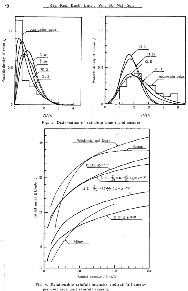
Count and amount distribution of raindrops Let compare with observation values and calculated values on probable density of raindrop counts /n and intensity of rainfall fi. An example is picked up in Fig. 5.

Energy equation We will obtain energy equations from eq. (30),(34),(35)and Table ２ in two cases (1.1) and (1.2).

Ｅ/Eo＝(が/2)cr5.5/√'4.5)〔(6/π)(r,.5/r4.5>'゜〕I/3＝14.0f0.１ａｉ (36) Ｅ/Eo＝(りV2)(r2.75/r2.25)〔(6/π')Cro.is/r2.'is^pi゜ｙ3＝10.6z｀0.137 (37)

The other cases ￡/￡o are obtained in Fig. 4.

０ｎ the relationship between rainfall energy and rainfall intensity several papers had been published.･

(8)

1.0 ″ り０／ l ｕｎｏｏ 1 0 Ｘ ; i ｓｕ 3 i ︶ａ t ＱＥ︵一〇Ｊｄ００１ ₂ Ｄ/Ｄｏ３ 1.0 0 1 5 ﹄７ｓｕｉｎｉＯＡ 1 0 A j i ｓｕａｐｇ t ＱＥＱＯ j ｊ０４０１２

Fig. 5. Distribution of raindrop counts and amount.

3 0 2 5 2 0 ︵日日 Z U J ／ｆ︶３Ａ３ｊａｕａ r i E i ｕｒｅｙ 15 12 3 D/Ｄo 0 50 100 Rainfallintensityバｍｍ/h)

Fig. 6. Relationship rainfall intensity and rainfall energy perunit area･ unit rainfall amount.

150

(9)

19

The eq. (38) had been proposed by Wischmeier and Smith'' which is famous for the element of rainfall factor to predict annual soil erosion loss from farm land.

E'Cst･foot/acre･inch) = 916 + 3311og /' (inch) (38) Exchanging to metric system it become eq. 閤.

Ｅ/E0 = 0.02636￡'=8.725(1.363+log O G9) Other investigator's results" translated into numerical equations from those graphical curves are as follows;

Hudson Ｅ/Ｅｏ＝29〔1−1/ＥＸＰ〔0.2 0o.e2〕 Ker E/￡o=13.5 j0.12

Mihara Ｅ/￡o＝8.0 ;o.2i

Our estimation values of､rainfall energy are shown in Fig. 6 with other investigator's results.

Conclusion

From the distribution of raindrop counts and amounts, two equations in the. cases (1.1) and (1.2) will express observation data. On the rainfall energy, it seems that the equation in the case (1.1) showed approximately simlar to resuls in the case (2.1). And in the other cases (1.2) and (2.2), equations are expressed loosely Mihara's results｡

As the conclusion, we consider that our equations should be used depending on each considerations, for example, simplicity, logicality or a substitute of other investigator's equations.

References

1) Laws, J. O., Measurments of the fall-velocity of water-drops and rain droｐs, Ｔｒａｎｓ.Ainer. Ｃｅｏｐりｓ.Ｕｎｉｏｎ，22, 709―721,(1941)

2) Gunn, R. and G. D. Kinzer, The terminal velocity of fall for water droplets, J. Iぼet., 6, 243―248, (1949)

3) Marshall, J. S. and W. M. Parmer, The distribution of raindrops with size, J. Met., 5, 165―166, (1948)

4) Shiotsuki, Y., On the flat size distribution of drops from convective raincloudｓ, Ｊ. Ｍｅt. ＳｏｃＪａｐａｎ．51， 42―60, (1974)

5) Wischmeier, W. H. and D.D. Smith, Rainfall energy and its relationship to soil loss, Ｔｒａｎｓ. Ａｍｅｒ，Ｇｅｏがりｓ，ＪＪｎｉ・m,39(2), 285-291, (1958)

6) Smith, D.D. and W. H. Wischmeir ， Rainfall erosionＡｄｖａｎｃｅｓ i71 Agｒｏｎｏｉ。^ｙ,Ｕ. 109-148, (1962)