A Phase-Plane Trajectory Vector-Based Method for Real-Time Identification of Critical Machines

© 200● The Institute of Electrical Engineers of Japan. 1

IEEJ TRANSACTIONS ON ELECTRICAL AND ELECTRONIC ENGINEERING

IEEJ Trans 2018

Vol.●● No.● pp.●-●● DOI:

A Phase-plane Trajectory Vector Based Method for Real-time

Identification of Critical Machines

Songhao Yang

Non-member,

Masahide Hojo

Member,

Baohui Zhang

Non-member

(Manuscript received Oct. 26, 2017, revised Jan 20, 2018)

Critical Machines (CMs) identification is the first and most important step of Equivalent-Single Machine Infinite Bus (E-SMIB) based methods such as EEAC and SMIE for transient stability assessment and control. This paper presents a novel real-time CMs identification method based on the Phase-plane Trajectory Vector (PTV) with PMU information support. The proposed method overcomes the drawbacks of conventional CMs identification methods and enables to track the change of CMs during the dynamic process. Only two sample points of all generators from PMUs are required to obtain the PTVs at each moment and the computation of feature matrix, as well as the k-means clustering, is fast and accurate. The application of the PTV based method is verified through cases study in IEEE 39 bus New England power system. Results are compared well with those obtained by conventional methods.

Keywords: Critical machine identification, phase-plane trajectory vector, real-time, transient stability, PMU

1. Introduction

The transient stability analysis of a power system, when subjected to a large disturbance, has always been an important issue. Extensive research activity has been being pursued on solving this problem, resulting in various analysis approaches, among which the method of Extend Equal Area Criterion (EEAC) [1-3] and SIngle Machine Equivalent (SIME) method [4-6] play a significant role. These hybrid methods have a wide application in offline and online transient stability assessment for their high accuracy and good adaptability. In these methods, all generators are first separated into two groups: the critical machines (CMs) group and the non-critical machines (NMs) group. The dynamic performance of multi-machine power system is then represented by the relative motion of two equivalent generators. And an Equivalent Single Machine Infinite Bus (E-SMIB) system is further presented to analyze the transient stability of the original system. In the application of E-SMIB based methods, the identification of CMs is of vital importance to the accuracy and validity of transient stability analysis [7]. Improper CMs identification may lead to delayed or even wrong transient stability detection result and invalid emergency control. A systematic method featuring a rapid and accurate CMs identification is thus necessarily required.

To realize the correct CMs identification, two features of CMs must be considered. The first feature is that the CMs change with disturbances and operation conditions. Now that it is not practical to assume all possible disturbances and operations in advance by offline simulation, the CMs identification should be better based on online simulation or real-time measurements. The second feature,

though few references referred, does exist that CMs may be variable during the whole dynamic process. It can be observed that some generators belong to NMs group after the disturbance but change to CMs group eventually, or vice versa. It is common in practical cases because continuous changes of system conditions (i.e. multiple faults) occur in the power system [8]. To track the time-evolution of CMs, the identification method is suggested to be carried out in real time.

Conventionally, critical machines are identified by examining the relative swing curves between machines. However, it is computationally time-consuming to verify all possible combination of generators because there are 2n-1_{possible combinations for a}

system with machines. In [6-7], a significant reduction in combination numbers is realized by the sorted angles of generators. The machines are separated by the largest angle gap (LAG) between two adjacent machines at a short time after disturbance clearance. Although the conventional LAG method is independent of disturbances and system operations, the time of CMs identification is difficult to choose and the identification results are inaccurate in some cases. Moreover, the result of CMs identification result by this method is fixed for each case and it can’t capture the change of CMs during the dynamic process.

Additionally, it is found that the identification of CMs and NMs is similar to the identification of coherent generators to some extent. The generators in CMs (NMs) behavior similar but they have an obviously different dynamic performance with those in NMs (CMs), which is similar to the issue of coherency identification. One major difference is that the number of generator groups is fixed to two in CM identification while it is not limited in coherency identification. Thus, the methods for coherency identification have a potential to identify the CMs. Two kinds of methods are mainly reported in references of coherency identification: the model-based methods and measurement based methods [9]. The model-based methods, such as the slow-coherency identification method [10-11], neglect the effects of variable system operating conditions and configuration which yet can alter the system coherency. The a) Correspondence to: Masahide Hojo.

E-mail: masa_hojo@tokushima-u.ac.jp ＊

State Key Laboratory of Electrical Insulation and Power Equipment, Xi’an Jiaotong University, Xi’an, 710049, China ＊＊

Department of Electrical and Electronic Engineering,

Tokushima University, 2-1 Minami-josanjima, Tokushima 770-8506, Japan

Paper

This is the peer reviewed version of the following article: Yang, S., Hojo, M. and Zhang, B. (2018), A phase‐plane trajectory vector‐based method for real‐time identification of critical machines. IEEJ Trans Elec Electron Eng, 13: 1578-1585., which has been published in final form at https://doi.org/10.1002/tee.22722. This article may be used for non-commercial purposes in accordance with Wiley Terms and Conditions for Use of Self-Archived Versions.

coherent generators identified by model-based methods keep unchanged when subjected to different disturbances under different system conditions, which is apparently improper for CMs identification. The measurement based methods, such as fast Fourier transform [12-13], empirical mode decomposition with the Hilbert transform [14], graph theory [8,15], support vector clustering [16], k-means clustering [17], and principal component analysis [18-19], can adapt to different disturbances and system conditions. However, they either need excessive computation, enormous training effort or wide time window. Moreover, these methods still fail to track the time-evolution of CMs during the dynamic process.

Motivated by these challenges, we propose a phase-plane trajectory vector (PTV) based CMs identification method which can be used in real time for transient stability detection. This method has advantages include 1) independence on disturbances and system operating conditions for its basis of PMU information, 2) less requirement of PMU data: 2 samples data are enough for CM identification of each moment and 3) ability to track the time-evolution of CMs during the dynamic process. This paper is organized as follows. The procedure of the proposed PTV method is described in Section II. Section III presents 3 detailed cases study of proposed PTV method applied to the IEEE 39 bus system. Section IV compares the proposed method with conventional methods and analyses the importance of real-time CMs identification. Section V concludes the paper.

2. Phase-plane trajectory Vector based method for

real-time CMs identification

2.1 Feature selection of phase-plane trajectory vectors

For a power system with N generators, the motion equation of i-th generator can be described as

0 , , , , 1, 2,..., i i i J i m i e i i d dt i N d M P P D dt  _{ }  _  _{ }  _   _{   }  (1),

where ,i i,P ande i, Pm i, are separately generator’s synchronous

angle, angular velocity deviation, electric power, and mechanical power. Parameters D is the damping factor and MJ i,is the inertia

moment. The angle and the angular velocity deviationi i describe the current state of the generator, which are controlled by regulators such as AVR, governor, PSS. The dynamic performance of a generator can be visible on the phase plane where the x-axis is the angle and the y-axis is the angular velocity. Each phase point





First of all, the relative motion among generators attracts more attention in the CMs identification. The Centre Of Inertia (COI) processing is necessary to analyze the relative dynamic performance of generators [20]. The angle and angular velocity deviation of the COI are defined as

, , 1 1 , , 1 1 ( ) ( ) ( ) , ( ) N N J i i J i i i i COI N COI N J i J i i i M t M t t t M M          









It is noted that the COI is time-varying which is decided by state variables. Thus the motion of each generator relative to the COI is

obtained by

( ) ( ) ( ), ( ) ( ) ( )

i t i t COI t i t i t COI t

        (3).

The Phase-plane trajectory Vector (PTV) is the vector from the point









the motion state and the trend of the i-th generator. t is the time interval of sample points from PMUs. Two sample points are required to obtain each PTV, each of which includes the information of generators’ angle and angular velocity deviation. For a power system with N generators, the number of PTVs obtained at each moment is N. Fig. 1 shows the PTVs on the phase plane, by which it is clear to identify the differences among different generators. As it is shown in Fig. 1, two following features are necessary to determine the motion of each PTV:

PTV location. The location of PTV indicates the angle and angular velocity deviation of generators, which are important for CMs identification. The location of generators is available by

1 1 2 2 ( ) ( ) ( ) ( ) [ ] ( ) ( ) N N t t t t t t           _    _{ }  _    θ Δω (4).

Fig. 1 The Phase-plane Trajectory Vector on the phase plane

-0.10 -0.05 0.00 0.05 0.10 -0.003 -0.002 -0.001 0.000 0.001 0.002 0.003 _ _ _ Quadrant III Quadrant II Quadrant IV  (p .u .) (rad) Quadrant I _

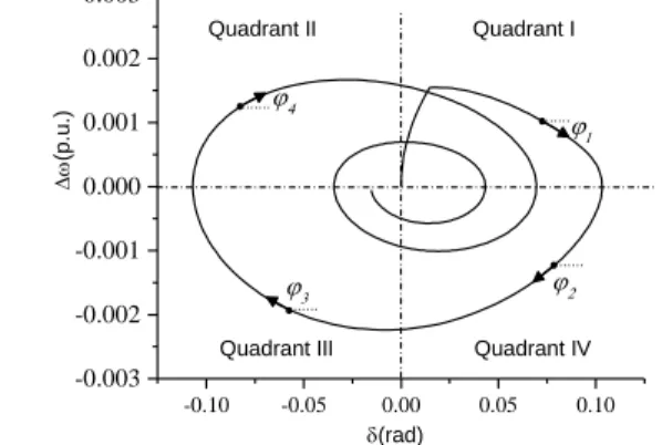
Fig. 2 The motion of PTV on the phase plane Table 1 The PTV angle and Generator state PTV angle Quadrant Range Generator State

1

 I (   ) 0,  0 (0, 2) Swing forward

2

 VI (   ) 0,  0 (2, ) Swing back

3

 III (   ) 0,  0 (2, ) Swing back

4

 II (   ) 0,  0 (0, 2) Swing forward PTV angle. The angles of PTVs relative to the positive x-axis represent the motion trend of generators. Taking motion trend into consideration can make the CMs identification faster and more accurate. The feature of PTVs angles can be obtained by(5):





Songhao Yang, Masahide Hojo and Baohui Zhang

3 IEEJ Trans. ●●, Vol.●●, No.●, ●●●

The motion angle of each PTV is computed by(6): ( ) arccos( i ) i i p e t p e   (6) where pi( ( )i t i(t  t), i( )t  i(t t)),e(1,0) . From (6), the value range of the PTV angle is (0, ) . The PTV angle is variable during the dynamic process, shown in Fig. 2. The figure shows the motion of the PTV of one generator when subjected to a large disturbance. The clockwise moving PTV indicates that the generator leaves the stable operating point and moves towards the new stable equilibrium point. Table 1 shows the value of is i corresponding to the generator state. When the PTV locates in upper half part of the phase plane, the generator swings forward, during which the value of is in range of (0, / 2)i  . And if the PTV locates in lower half part of phase plane, the generator swings back and the value of is in range of ( / 2, )i   .

The feature matrix of PTVs is thus obtained as

[ ]



A θ Δω φ (7).

The matrix A represents the features of PTVs, by which

generators can be divided into two groups: CMs and NMs. Different from other CMs identification methods, proposed method not only focus on the angle but also pay attention to the angular velocity and motion trend, which indicates the future motion of generators by(1). Proposed PTVs describe much more information than the angle curves of generators. It is also noted that A is time-varying,

which is computed with PMU information at each moment. By the real-time updated feature matrix, PTVs describe the dynamic performance of generators visibly. The time-evolution of CMs can thus be tracked by PTVs.

2.2 PTV based real-time identification of CMs

To identify the CMs and NMs, the K-means clustering method is applied. K-means clustering method is popular for cluster analysis in data mining. It has the advantages of little computation, fast clustering and high accuracy. The difficulty of K-means clustering method is to determine K-the number of coherent groups. However, K is fixed to 2 in the special scenario of CMs identification. Following simulations also verify the applicability of K-means clustering in this paper.

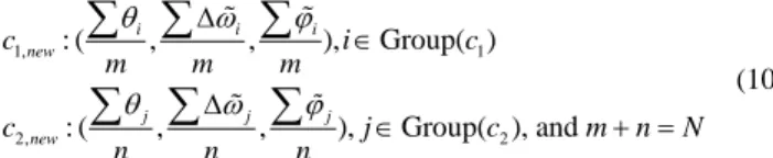
The details of K-means method can be available from literature [16]. Firstly, two clustering centers are given at the beginning as:

1: ( c1, c1, c1)

c    and c2: (c2, c2, c2) . For a fast calculation,

the initial centers are selected as the generator with the largest angle and the one with the least angle. Then the distance from generators to each clustering center is computed with the feature matrix. To balance the impact of each feature on distance computation, the units for i( ),t i( ) and t i( )t are rad, p.u. and rad/π. The new feature matrix of PTVs at each moment is:

[ ] [ / ]

 

A θ Δω φ θ Δω φ (8) The Euclidean distance is used to measure the distance of i-th generators to the two cluster centers:

2 2 2 1 1 1 1 2 2 2 2 2 2 2 ( , ) ( ) ( ) ( ) ( , ) ( ) ( ) ( ) i c i c i c i c i c i c dis i c dis i c                             (9)

Generators are assigned to the group of closer clustering center. For example, i-th generator belongs to the group C1 if

1 2

( , ) ( , )

dis i c dis i c . By this way, generators are divided into two groups. New clustering centers are obtained by these two groups:

1, 1 2, 2 : ( , , ), Group( ) : ( , , ), Group( ), and i i i new j j j new c i c m m m c j c m n N n n n            

 



 



where m and n are separately the number of generators in Group(C1) and Group(C2). New distances are computed and the cycle process continues until the clustering result remains unchanged. The group with larger inertia is usually regarded as the CMs and the rest group is NMs.

The overall procedure for real-time CMs identification can be summarized in the following steps:

step 1. Read real-time information from PMUs which includes the angle, angular velocity deviation of generators of current moment;

step 2. Make the COI processing of original information and initialize the data by subtracting the stable operation state information;

step 3. Check whether generators are out-of-step by angle threshold (i.e. 2π). If the angle of the generator is larger than the threshold, this generator is marked as the out-of-step generator;

step 4. Obtain the feature matrix A of rest generators at

moment t by (8);

step 5. Apply the K-means clustering method based on the feature matrix A and output the CMs identification results;

step 6. Return to step 1 and keep tracking the change of CMs until the system runs to a new stable operating point. The following sections present the results obtained by applying the PTV based method to a tested system.

3 Study Results

Fig. 3 New England 39 bus test power system

In this section, the proposed PTV based method for CMs identification is tested in the New England 39 bus 10 machines power system as shown in Fig. 3 [8]. The generators of tested power system adopt the two-axis generator model equipped with AVRs and PSSs. The dynamic of the system is simulated on the PSASP- a platform for transient simulation and analysis. The time interval of output data is 10ms, which is regarded as the PMU information in the real-time CMs identification scheme. Many cases have been simulated, however, only three typical cases are presented here to show the validity of the proposed method.

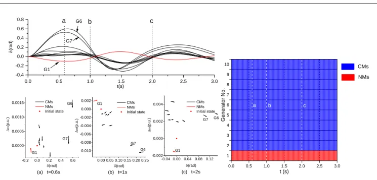
Vol.●● No.● pp.●-●● DOI: 0.0 0.5 1.0 1.5 2.0 2.5 3.0 -0.4 -0.2 0.0 0.2 0.4 0.6 0.8 -0.2 0.0 0.2 0.4 0.6 0.0000 0.0005 0.0010 0.0015 0.00 0.05 0.10 0.15 0.20 0.25 -0.010 -0.008 -0.006 -0.004 -0.002 0.000 0.002 -0.04 0.00 0.04 0.08 0.12 -0.002 0.000 0.002 0.004 G7 G6 (r ad) t(s) G1 G7 G6 G1 CMs NMs Initial state  (p.u.) (rad) G7 G6 G1  (p.u.) (rad) CMs NMs Initial state (c) t=2s (b) t=1s G7 G6 G1  (p.u.) (rad) CMs NMs Initial state (a) t=0.6s a b c

Fig. 4 Generator angle curves and the PTVs at different moments in Case 1. Fig. 5 The CMs identification results in Case 1

0.0 0.5 1.0 1.5 2.0 2.5 3.0 -5 0 5 10 15 20 -0.5 0.0 0.5 1.0 1.5 2.0 2.5 -0.02 -0.01 0.00 0.01 0.02 0.03 0.04 0.05 -1 0 1 2 3 4 -0.01 0.00 0.01 0.02 0.03 0.04 0.05 0.06 -2.8 -2.7 -2.6 -2.5 -2.4 -2.3 -0.020 -0.019 -0.018 -0.017 -0.016 -0.015 -0.014 -0.013 -0.012 (c) t=2.5s (b) t=2s (rad ) t(s) G6,G7 G5 a b c (a) t=1.2s G5  (p.u.) (rad) CMs NMs Initial state G6 G7 CMs NMs Initial state  (p.u.) (rad) G5 CMs NMs  (p.u.) (rad) G4

Fig. 6 Generator angle curves and the PTVs at different moments in Case 2 Fig. 7 The CM identification results in Case 2

Fig. 8 Generator angle curves and the PTVs at different moments in Case 3. Fig. 9 The CM identification results in Case 3 0.0 0.5 1.0 1.5 2.0 2.5 3.0 1 2 3 4 5 6 7 8 9 10 c b t (s) Gen er ato r No . NMs CMs a 0.0 0.5 1.0 1.5 2.0 2.5 3.0 1 2 3 4 5 6 7 8 9 10 c b t (s) Gen era tor No. CMs NMs Out of step Generator a 0.0 0.5 1.0 1.5 2.0 2.5 3.0 -1 0 1 2 -0.05 0.00 0.05 0.10 0.15 0.20 0.25 -0.010 -0.008 -0.006 -0.004 -0.002 0.000 0.002 -0.1 0.0 0.1 0.2 0.3 0.4 0.5 0.6 0.7 0.8 0.9 0.000 0.002 0.004 0.006 0.008 0.010 2nd Disturbance (rad) t(s) G1 G9 a _b 1st Disturbance G9 (rad) CMs NMs Initial state G1

Generator Angle Curves

(b) t=2.5s (rad) CMs NMs Initial state (a) t=1s 0.0 0.5 1.0 1.5 2.0 2.5 3.0 1 2 3 4 5 6 7 8 9 10 b t (s) Gen er ato r No . CMs NMs a

Songhao Yang, Masahide Hojo and Baohui Zhang

5 IEEJ Trans. ●●, Vol.●●, No.●, ●●●

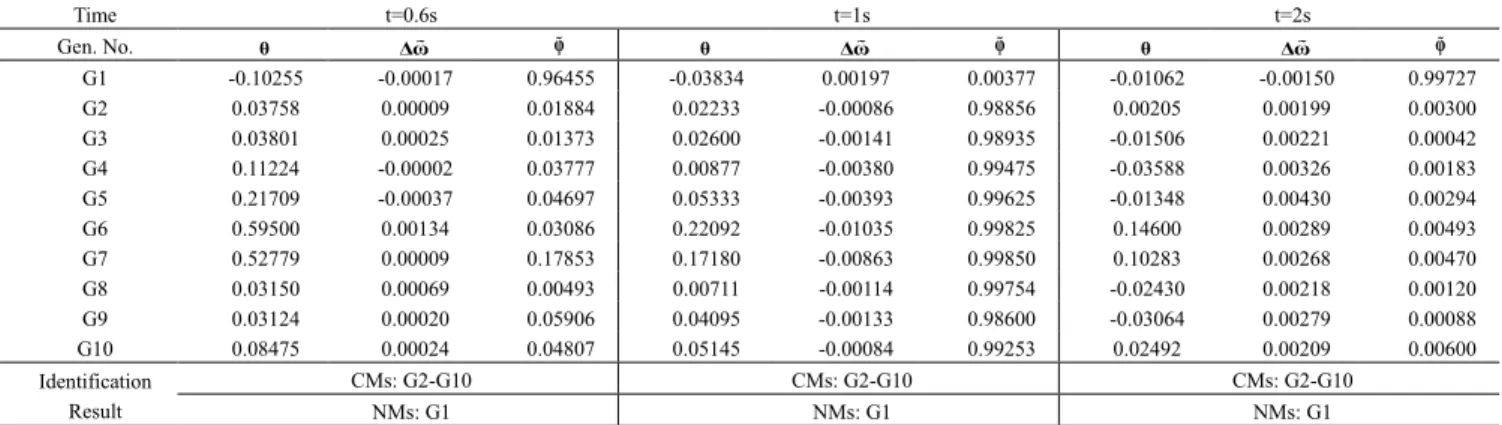
Table 2 Feature Matrix at different times and CMs identification results in Case 1

Time t=0.6s t=1s t=2s Gen. No. G1 -0.10255 -0.00017 0.96455 -0.03834 0.00197 0.00377 -0.01062 -0.00150 0.99727 G2 0.03758 0.00009 0.01884 0.02233 -0.00086 0.98856 0.00205 0.00199 0.00300 G3 0.03801 0.00025 0.01373 0.02600 -0.00141 0.98935 -0.01506 0.00221 0.00042 G4 0.11224 -0.00002 0.03777 0.00877 -0.00380 0.99475 -0.03588 0.00326 0.00183 G5 0.21709 -0.00037 0.04697 0.05333 -0.00393 0.99625 -0.01348 0.00430 0.00294 G6 0.59500 0.00134 0.03086 0.22092 -0.01035 0.99825 0.14600 0.00289 0.00493 G7 0.52779 0.00009 0.17853 0.17180 -0.00863 0.99850 0.10283 0.00268 0.00470 G8 0.03150 0.00069 0.00493 0.00711 -0.00114 0.99754 -0.02430 0.00218 0.00120 G9 0.03124 0.00020 0.05906 0.04095 -0.00133 0.98600 -0.03064 0.00279 0.00088 G10 0.08475 0.00024 0.04807 0.05145 -0.00084 0.99253 0.02492 0.00209 0.00600 Identification Result CMs: G2-G10 CMs: G2-G10 CMs: G2-G10 NMs: G1 NMs: G1 NMs: G1

Table 3 Feature Matrix at different times and CMs identification results in Case 2

Time t=1s t=2s t=2.5s Gen. No. θ Δω φ θ Δω φ θ Δω φ G1 -0.10255 -0.00017 0.96455 -1.20475 -0.01113 0.997498343 -2.37493 -0.01366 0.9999 G2 0.03758 0.00009 0.01884 -1.39163 -0.00937 0.997574444 -2.43081 -0.01378 0.9971 G3 0.03801 0.00025 0.01373 -1.42900 -0.00860 0.999138786 -2.43873 -0.01480 0.99688 G4 0.11224 -0.00002 0.03777 -1.48788 -0.00214 0.939128812 -2.77802 -0.01784 0.9984 G5 0.21709 -0.00037 0.04697 4.04855 0.06060 0.003082456 - - - G6 0.59500 0.00134 0.03086 - - - - G7 0.52779 0.00009 0.17853 - - - - G8 0.03150 0.00069 0.00493 -1.4425 -0.00763 0.996791332 -2.47063 -0.01460 0.99719 G9 0.03124 0.00020 0.05906 -1.45613 -0.00778 0.99948356 -2.40175 -0.01363 0.99598 G10 0.08475 0.00024 0.04807 -1.35483 -0.00804 0.997597503 -2.37230 -0.01568 0.99793 Identification Result

Out of Step Generators: None Out of Step Generators: G6, G7 Out of Step Generators: G5-G7

CMs: G6-G7 CMs: G5 CMs: G4

NMs: G1-G5, G8-G10 NMs: G1-G4, G8-G10 NMs: G1-G3, G8-G10 Table 4 Feature Matrix at different times and CMs identification results in Case 3

Time t=1s t=2.5s Gen. No. θ Δω φ θ Δω φ G1 -0.03834 0.00197 0.00377 -0.13840 -0.00047 0.99144 G2 0.02233 -0.00086 0.98856 0.07721 -0.00088 0.98272 G3 0.02600 -0.00141 0.98935 0.09052 -0.00095 0.98402 G4 0.00877 -0.00380 0.99475 0.12316 -0.00063 0.97833 G5 0.05332 -0.00393 0.99625 0.18755 -0.00080 0.97853 G6 0.22091 -0.01035 0.99825 0.30742 -0.00014 0.96302 G7 0.17180 -0.00863 0.99850 0.25197 -0.00001 0.91282 G8 0.00711 -0.00114 0.99754 0.06945 -0.00085 0.99071 G9 0.04094 -0.00133 0.98600 0.91754 0.01045 0.00383 G10 0.05145 -0.00084 0.99253 0.10929 -0.00026 0.90549 Identification Result CMs: G2-G10 CMs: G9 NMs: G1 NMs: G1-G8, G10 Table 5 Comparison of PTV method with other methods for CMs identification in Case 1

Time t=0.6s t=1.2s t=2.5s t=4.2s

Conventional LAG method CMs:{G2-G9} NMs:{G1,G10} Real-time LAG method CMs:{G6,G7}

NMs:{G1-G5,G8-G10} CMs:{ G4-G7 } NMs:{ G1-G3,G8-G10 } CMs:{G2-G10} NMs:{G1} CMs:{G6,G7} NMs:{G1-G5,G8-G10} PTV method CMs:{G2-G10} NMs:{G1} CMs:{G2-G10} NMs:{G1} CMs:{G2-G10} NMs:{G1} CMs:{G2-G10} NMs:{G1} Correct CMs and NMs CMs: {G2-G10} NMs: {G1} 3.1 Case 1

In case 1, a three-phase short circuit ground fault occurs in the middle of transmission line 21-22 at 0s, and then the fault line is eliminated at 0.1s. The system is transient stable eventually and the angle curves of generators are shown in Fig. 4. The CMs identification results are shown in Fig. 5.

In Fig. 5, the groups to which each generator belongs are distinguished by different colors. The Blue blocks stand for the CMs while the Red blocks stand for the NMs. From Fig. 5, there is only one mode of CMs and NMs during the whole dynamic process: group {G1} and group {G2-G10}. Fig. 4 also shows the figures of PTVs at different moments such as 0.6s, 1s and 2s. These moments

are selected because either angles or angular velocity deviation are similar and misidentification is easy to obtain by other CMs identification methods (which will be further discussed in section 4). However, the figures of PTVs show obvious differences on the locations or the motion trend between CMs and NMs. The initial state in Fig. 4 is the (0,0) in phase plane, standing for the stable operation point of generators before the disturbance. The feature matrices A of these moments are presented in Table 2. During the whole dynamic process, the CMs and NMs identification result keeps unchanged: the CMs are {G2-G10} and NM is {G1}, which is identical to above analysis. The excellent performance of PTV method in case 1 benefits from the typical features selected which well describes the dynamic behavior of generators.

3.2 Case 2

In case 2, same three-phase short circuit ground fault occurs on the transmission line 21-22 at 0s, and the fault line is eliminated at 0.2s. Due to the delayed relay operation, the system is unstable eventually and the angle curves of generators are shown in Fig. 6. The CMs identification results are shown in Fig. 7.

In Fig. 7, generator groups are distinguished by different colors. The blue blocks stand for the CMs while the red blocks stand for the NMs. These out-of-step generators are especially represented by black blocks. The time-evolution of generator groups are clearly observed in Fig. 7. G1 is the NM and rest generators are CMs at first after the fault clearance in the period of 0-0.66s. G6 and G7 become CMs later in the period of 0.67s-1.58s. The angles of G6 and G7 increase continuously and become out-of-step after 1.59s. Then G5 is identified as CM in the period of 1.59s-2.21s. After 2.22s, G5 become out-of-step and G4 is identified as CM. This time-evolution of CMs often occurs in transient unstable cases. Influenced by unstable machines, some machines in NMs change to the CMs and become out-of-step eventually. Conventional methods fail to identify the changes of CMs in such cases. However, the time-evolution of CMs are tracked successfully by the proposed PTV method thanks to its ability of real-time identification. As it is shown in Fig. 7, different CMs are identified by the PTVs at different moments. The feature matrices and identification results are summarized in Table 3.

3.3 Case 3

Two continuous disturbances are simulated in the case 3. The first three-phase short circuit ground fault occurs on the line 21-22 at 0s, and then the fault line is eliminated at 0.1s. Afterward, the second three-phase short circuit ground fault occurs on line 28-29 at 2s, and then the fault line is eliminated at 2.1s. The angle curves of generators and PTVs at different times are shown in Fig. 8 and CMs identification results are given in Fig. 9.

Before the occurrence of the second disturbance, CMs in case 3 are same to that in case 1. However, the second disturbance changes the stability of power system and influences the mode of CMs and NMs. G9 begins to accelerate and becomes unstable eventually. Fig. 9 shows the evolution of CMs in Case 3. CMs are {G2-G10} in period of 0-2.4s and change to {G9} in period of 2.41s-3s. The feature matrix and identification results of different moments are presented in Table 4. The changes of CMs are identified correctly via the proposed method.

4 Discussion

4.1 Comparison with other CMs identification methods

As is referred in the introduction, the most popular method for

CMs identification is the largest angle gap (LAG) method which is widely used in SIMB based methods such as EEAC and SIME. This method can identify the CMs with the information of generator angles at a certain time soon after the clearance of disturbances. However, the time for information selection is not easy to decide. If the time is too early, the angles of generators are similar, as a result of which the CMs identification result is greatly influenced by the initial state. In this case, the CMs identification result will be inaccurate. On the other hand, if the time is too late, transient stability detection will be delayed. Literature [6] adopts the identification time as 100ms after the disturbance elimination, but the accuracy of CMs identification still can’t be guaranteed. Moreover, the identification result of the conventional LAG method is fixed for each case and it fails to track the change of CMs during the dynamic process.

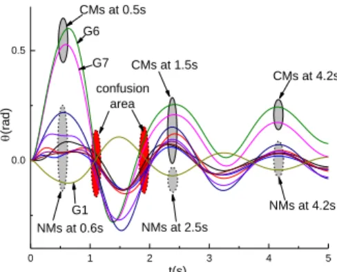
Inspired by the measurement based coherency identification methods, the conventional LAG method can be modified to apply in real time [21]. To eliminate the influence of the initial state, the same initialization proceeding as PTV methods is necessary. The clustering process is carried out at each moment with PMU information and CMs identification result is updated in real time. This real-time LAG method has better performance than the conventional LAG method because it can identify the changes of CMs during the dynamic. For example, the change of CMs in case 2 and case 3 can also be identified by the real-time LAG method. However, it arises some new troubles. As it is shown in Fig. 10, the application of the real-time LAG method in case 1 is not ideal. There is some confusion area for the modified LAG method where the CMs swing back and the angles of CMs are similar with that of NMs. The CMs identified by the real-time LAG method are not accurate at that time.

The comparison of the conventional LAG method, real-time LAG method and proposed PTV method are presented in Table 5. The correct CMs of case 1 are always {G2-G10} from observation. The CMs identification result of the conventional LAG method is fixed as {G2-G9} which are not correct. Although the real-time LAG method identifies the CMs correctly at 2.5s, it fails to identify the correct CMs at 0.6s and 4.2s. The identification results in confusion area in Fig. 10 are even worse when CMs swing back. On the contrary, the proposed PTV method correctly identifies the CMs at all these moments. The PTVs in Fig. 4 show obvious differences between CMs and NMs, especially in the confusion area. Results in Table 5 indicate the feature matrix of PTVs are useful to distinguish the CMs and NMs.

0 1 2 3 4 5 0.0 0.5 NMs at 4.2s CMs at 1.5s NMs at 2.5s NMs at 0.6s G7 G6 (r ad ) t(s) G1 CMs at 0.5s confusion area CMs at 4.2s

Fig. 10 The real-time largest angle gap method for CMs identification

Songhao Yang, Masahide Hojo and Baohui Zhang

7 IEEJ Trans. ●●, Vol.●●, No.●, ●●●

4.2 The real-time identification for CMs

In general, the CMs are not identified in real time in literature because the E-SMIB based methods are usually applied in offline transient stability analysis. Even in the online application, the CMs are identified once after disturbances clearance and the CMs identification result is fixed for each case. As a result, changes of CMs during the dynamic are ignored in these studies. With the development of WAMS in the power system, researchers try to extend the E-SMIB based methods to real-time transient stability detection and control. Aspired by this aim, the method of EEAC is developed to the DEEAC [22] and SIME method is developed to the predictive SMIE method [6]. Real-time prediction and parameters update is the key to obtain an accurate real-time SMIB. The method of CMs identification, as the first step of E-SMIB, also need to be improved to apply in the real-time scenario.

The real-time identification of CMs puts forwards a high request to the identification method with fast computation, less information requirement and high accuracy. Proposed PTVs method succeeds in meeting these requirements:

o The computation of PTVs and the K-means clustering are simple and fast. The average calculation time of tests cases of IEEE 39 bus 10 machine power system is 3ms including the data processing and k-means clustering. The calculation is done with MATLAB R2013a on a computer with Intel i5 CPU. The results are believed to be further improved on a better computation platform.

o For each moment, only two sample points of all generators are necessary to obtain all the PTVs. The necessary information includes the angle θ and angular speed  . These variables 

can be obtained directly or indirectly from PMUs. For example, the angles of generators δ are provided by PMUs [23]. And the angular speed ∆ω is computed by the output frequency fi of generators from PMUs:

0 0 0 0 i i i f f f          (11)

In (11), f0is the synchronization frequency of power system, i.e.

50Hz or 60Hz. And then δ and ∆ω are further processed by (2) and (3) to obtain the angle θ and angular speed  relative to the COI.  The less requirement for information makes the method more reliable.

5 Conclusion

This paper proposes a novel method for real-time CMs identification. This method is based on the PTVs, of which the feature matrix is used to describe the dynamic of generators. K-means clustering method is used to separate the generators into two groups: CMs and NMs on the basis of the feature matrix. The PTVs are obtained with PMU information and the identification result is updated in real time. The simulations in test system show that the proposed method is more accurate than conventional methods in general cases. Moreover, the PTV based method can track the change of CMs. The proposed method can provide an accurate CMs identification result at each moment and track the time-evolution of CMs during the dynamic process with PMU information. Combined with E-SIMB based method such as EEAC and SIME, this real-time CMs identification method will facilitate the study of real-time transient stability detection and control.

References

(1). Xue, Y., Van Custem, T. and Ribbens-Pavella, M.: Extended equal area criterion justifications, generalizations, applications, IEEE Transactions on Power System, 1989, 4, (1): 44-52

(2). Xue, Y., Van Cutsem, T. and Ribbens-Pavella, M.: A simple direct method for fast transient stability assessment of large power systems, IEEE Transactions on Power System, 1988, 3, (2): 400-412

(3). Xue, Y., Van Cutsem, T. and Ribbens-Pavella, M.: Real-time analytic sensitivity method for transient security assessment and preventive control, IEE Proceeding Generation, Transmission and Distribution, 1988, 135, (2): 107-117 (4). Ernst, D., Ruiz-Vega, D. and Pavella, M.: A unified approach

to transient stability contingency filtering, ranking and assessment, IEEE Transactions on Power System, 2001, 16, (3): 435-443

(5). Miah, A. M.: Simple dynamic equivalent for fast online transient stability assessment, IEE Proceeding Generation, Transmission and Distribution, 1998, 145, (1): 49-55 (6). Pavella, M., Ernst, D. and Ruiz-Vega, D.: Transient stability

of power systems: a unified approach to assessment and control (Kluwer Academic Publishers, 2010)

(7). Xue, Y. and Pavella, M.: Critical-cluster identification in transient stability studies, IEE Proceeding Generation, Transmission and Distribution, 1993, 140, (6): 481-489 (8). Gomez, O. and Rios, M. A.: Real time identification of

coherent groups for controlled islanding based on graph theory, IET Generation, Transmission and Distribution, 2015, 9, (8): 748-758

(9). Khalil, A. M. and Iravani, R.: A Dynamic Coherency Identification Method Based on Frequency Deviation Signals, IEEE Transactions on Power System, 2016, 31, (3): 1779-1787

(10). De Tuglie, E., Iannone, S. M. and Torelli, F.: A coherency recognition based on structural decomposition procedure, IEEE Transactions on Power System, 2008, 23, (2): 555-563 (11). Yusof, S. B., Rogers, G. J. and Alden, R.: Slow coherency

based network partitioning including load buses, IEEE Transactions on Power System, 1993, 8, (3): 1375-1382 (12). Jonsson, M., Begovic, M. and Daalder, J.: A new method

suitable for real-time generator coherency determination, IEEE Transactions on Power System, 2004, 19, (3): 1473-1482

(13). Vahidnia, A., Ledwich, G. and Palmer, E.: Generator coherency and area detection in large power systems, IET Generation, Transmission and Distribution, 2012, 6, (9): 874-883

(14). Avdakovic, S., Becirovic, E. and Nuhanovic, A.: Generator Coherency Using the Wavelet Phase Difference Approach, IEEE Transactions on Power System, 2014, 29, (1): 271-278 (15). Najafi S, Hosseinian S H, Abedi M. Proper splitting of

interconnected power systems'. IEEJ Transactions on Electrical and Electronic Engineering, 2010, 5(2): 211-220. (16). Agrawal, R. and Thukaram, D.: Support vector

clustering-based direct coherency identification of generators in a multi-machine power system, IET Generation, Transmission and Distribution, 2013, 7, (12): 1357-1366

for coherency identification using an artificial neural network, IEEE Transactions on Power System, 1994, 9, (4): 2056-2062 (18). Ariff, M. A. M. and Pal, B. C.: Coherency Identification in Interconnected Power System- An Independent Component Analysis Approach, IEEE Transactions on Power System, 2013, 28, (2): 1747-1755

(19). Qing X, Wang S, Jia T, et al. Robust principal component analysis-based coherency identification of generators with missing PMU measurements'. IEEJ Transactions on Electrical and Electronic Engineering, 2016, 11(1): 36-42. (20). Cepeda, J. C., Rueda, J. L. and Colome, D. G.: Real-time

transient stability assessment based on centre-of-inertia estimation from phasor measurement unit records, IET Generation, Transmission and Distribution, 2014, 8, (8):

1363-1376

(21). Su, F., Zhang, B. and Yang, S.: Study on real-time clustering method for power system transient stability assessment. 2016 IEEE Power and Energy Society General Meeting (PESGM), July 2016

(22). Xue, Y., Huang, T. and Li, K.: An efficient and robust case sorting algorithm for transient stability assessment, 2015 IEEE Power & Energy Society General Meeting(PESGM), Denver, CO, USA, July 2015

(23). Yang Q, Bi T, Wu J. WAMS implementation in China and the challenges for bulk power system protection, 2007 IEEE Power & Energy Society General Meeting(PESGM): 1-6.

Songhao Yang (Non-member) He received the Bachelor Degree in

electrical engineering from Xi’an Jiaotong University in 2012 and is presently pursuing his Ph. D. degree in electrical engineering, Xi’an Jiaotong University. Meanwhile, he is also pursuing his Ph. D. degree in engineering at Tokushima University. His research interests are power system transient stability assessment & control and optimal PMUs placement.

Masahide Hojo (Member) He received the Ph.D. degree in

engineering from Osaka University in 1999 and is presently a professor at Tokushima University. His research interests are the advanced power system control by power electronics technologies and analysis of power systems.

Baohui Zhang (Non-member) He received the Ph.D. degree in

electrical engineering from Xi’an Jiaotong University in 1988 and is presently a professor at Xi’an Jiaotong University. His research interests are system analysis, control, communication, and protection.