Using Expert Knowledge to Alleviate the Lack of Data in Predictive Analytics: A Case Study of Estimating Electronic Components Failure Rate

全文

(1)情報処理学会第 80 回全国大会. 1C-04. Expert Knowledge for Alleviating Lack of Data: Estimating Electronic Components Failure Rate Matthieu Parizy1,a). 1.. Tatsuya Yamamoto1,b). Hiroshi Ikeda1,c). INTRODUCTION AND MOTIVATION. Being an electronic device maker, in order to satisfy our customers expectations regarding the quality of our products, we have to grasp the quality of the components we use. Until now, using the information in the specifications provided by the component maker as well as our component expert’s experience was our main way to evaluate the quality of those components. However, having accumulated over the years electronic components failure records when a device failed, we assumed that mining those records could help our experts getting a better grasp of components quality by finding links between the specifications and the failures. Thus, our main motivation for this work is to succeed in: ( 1 ) Identifying key factors in electronic components failure ( 2 ) Predicting failure rate of said components Applying machine learning techniques to small data is challenging due to the difficulty of avoiding overfitting. Our contribution is how we used an expert’s knowledge to reduce overfitting by having him sort by order of relevancy each explanatory variable to guide our stepwise model selection by AIC(stepAIC) [4] of our Generalized Linear Model(GLM) [2] in R[3] for one type of component and one type of failure. In cross-validation, our expert guided model shows an improvement of 130% when compared to the normalized root-mean-square deviation (NRMSD) of our non-expert guided model. We fill first present our data specificities, then our method of analysis and finally our results.. 2.. DATA SPECIFICITIES. As mentioned in the introduction, our data is what we qualify as "small", and is presented in table 1. We have available P to us around 100 failures ( f ≈ 100) of a certain type, spread over around 30 components (c with f , 0) plus 100 non failing components (c with f = 0) of a certain type. Each component’s specifications are expressed in the form of 30 variables which can be used as explanatory variables (n ≈ 30). . The ratio f /b gives us the observed fail rate pˆ of a given component c. One of our goal is to find the actual fail rate p but the below specificities of our data was problematic: • The non-null pˆ remains low in general ( pˆ < 0.00001) 1 a) b) c) d). Fujitsu Laboratories Ltd., 1-1, Kamikodanaka, 4-chome, Nakahara-ku, Kawasaki 211–8588, Japan [email protected] [email protected] [email protected] [email protected]. 2-19. Component Name c1 ... cm. Hidetoshi Matsuoka1,d). Table 1 Fail Records Response Bought Qty. Fail Qty. b1 f ... ...1 bm fm. Explanatory Variables Spec1 ... Specn s11 ... s1n ... ... ... snm ... snm. • Half of our data has a low bought quantity (b < 10000) Because of that, it is hard to estimate p since we have several components with a relatively high pˆ for a low bought quantity. We assumed that in those cases, it is highly likely that pˆ is far from p, cases which can be explained by having bought only a few lots of components including a bad one. Thus to fit those specificities, we decided to use GLM which can take into account this risk of pˆ being far from p.. 3.. METHOD OF ANALYSIS Build GLM with all variables. Perform stepAIC from full model. Perform stepAIC from empty model. Guide stepAIC with expert knowledge expressed as graded explanatory variables *1 Fig. 1. Our Approach. As summarized in figure 1, and mentioned in the previous part, we first built a GLM with every available explanatory variable available. This resulted in a poor model fit wise with a high mean squared error (MSE) and a high Akaike Information Criterion(AIC)[1] of 66000 compared to our following modeling attempts. To obtain a better model, we then performed a stepAIC on the previous GLM which also gave a high AIC of 69000 and MSE. Next step was to let stepAIC examine models with a scope starting from an empty formula to a formula containing all variables which finally yielded promising results with an AIC of 74. The problem this time was that some of the variables kept by the stepAIC were not satisfying for our expert as he deemed and explained that physically the kind of failure studied could not be linked in any way to some of the kept variables plus since our data set is small we were also afraid that our model would be too overfitted. Our final modeling attempt and our main contribution, was to Details in Algorithm 1. Copyright 2018 Information Processing Society of Japan. All Rights Reserved..

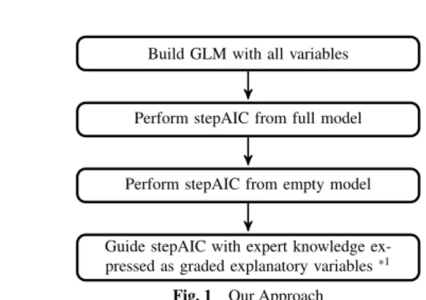
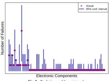
(2) 情報処理学会第 80 回全国大会. ●. Number of Failures. combine our expert’s knowledge by having him grade each potential explanatory variables from 1(no link to the kind of failure studied, should be pruned) to 5(very confident this variable is linked to this kind of failure) and to finally combine those graded explanatory variables in the stepAIC as shown in algorithm 1. Compared to previous models, it gave us an AIC of 104. Its results will be detailed in part 4 To identify the key factors in electronic components failure, during the various modeling phases, we recorded after each stepAIC modeling phases the kept variables with a significant pvalue(<0.05).. Actual 95% conf. interval. ●. ● ● ● ●. ●. ●● ● ●●●● ●●●● ● ●●●●●●●●●●●●●●●●●●●●●●●●●●●●●●●●●●●●●●●●●●●●●●●●●●●●●●●●●●●●●●●●●●. Algorithm 1 stepAIC combined with Expert Knowledge 1: 2: 3: 4: 5: 6: 7: 8: 9: 10: 11: 12: 13: 14: 15: 16: 17: 18:. procedure makeExpertModel input: data ← List of failureData exVarGraded ← set of graded explanatory variables output: GLM with variables chosen by stepAIC and exVarGraded main: currentGrade ← maxGrade(exVarGraded) while currentGrade ≥ minGrade(exVarGraded) do currentExVar ← {x ∈ exVarGraded | grade = currentGrade} currentModel ← glm(data, currentExVar) currentModel ← stepAIC(currentModel, keptExVar, currentExVar) if AIC(currentModel) ≥ prevAIC then return prevModel prevAIC ← AIC(currentModel) prevModel ← currentModel keptExVar ← var(currentModel) currentGrade ← currentGrade − 1 return currentModel. In order to combine the previously built GLM with our established explanatory variables grade, we conceived Algorithm 1: In descending order of grade importance(line 9 and line 17), we take the explanatory variables corresponding to current grade (line 10), make the GLM for those variables (line 11), select the best variables with stepAIC within current grade variables(line 12), and then check the resulting model’s AIC. If we reached a better model compared to the one built with the previously processed explanatory variables corresponding to the previous (higher) grade, we loop to process the variables in the grade below. If the previous model was better, we stop processing further and return this model (line 13).. 4.. RESULTS. 4.1 Fitting The p-value for some of our explanatory variables obtained after making our GLM showed was significant (p-value < 0.05). When we showed those results to our expert it allowed him to confront his own assumptions on what part of the specifications he thought was relevant for the studied failure type to those deemed significant GLM-wise. It revealed that the GLM was able to extract both matching and non-matching knowledge to our expert’s. For most of the non-matching cases, it highlighted the high proportion of outliers present in the available data and more importantly it led us to prune out those variables to reduce the risk of overfitting. For the matching cases, it reinforced the expert’s. 2-20. Electronic Components Fig. 2. Prediction confidence interval. confidence in his experience. We present in figure 2 the actual predicted number of failures (red dots) compared to the predicted number of failures within a 95% confidence interval for each of the components in our data. As we can observe, all the actual values fit within their predicted interval. Although not shown here, for our pure stepAIC based model, we had one component which actual value did not fit in its interval. 4.2 Cross-Validation Due to the lack of data, we chose a leave one out approach for our k-fold cross-validation. Since most of the components in our data has a low failure rate, we thought it would be relevant to compare our model’s MSE resulting from cross validation to a trivial model only predicting a failure rate of 0 for any components which we called Zero Model (ZM). It shows encouraging results: our EGM has an MSE almost five times better than the NEGM and 6.6% better than the ZM. NRMSD wise, EGM is twice better than NEGM and 3.3% better than ZM.. 5.. CONCLUSION. We successfully combined our expert’s knowledge with our small data to assess more accurately our components key factors in failures. We were also able to predict each components number of failures within a 95% interval of confidence with satisfying cross-validation results. Our future work will focus on applying this methodology to other electronic components and most importantly, we will build a framework where we accumulate expert knowledge and constantly confront it to available data in order for them to make more accurate decisions when considering buying new components. References [1] [2] [3] [4]. Akaike, H.: Akaike’s Information Criterion, Springer Berlin Heidelberg, Berlin, Heidelberg (2011). Dobson, A. J.: An Introduction to Generalized Linear Models, Chapman and Hall, London (1990). R Foundation for Statistical Computing: R: A Language and Environment for Statistical Computing, Vienna, Austria (2017). Venables, W. N. and Ripley, B. D.: Modern Applied Statistics with S, Springer, New York, fourth edition (2002).. Copyright 2018 Information Processing Society of Japan. All Rights Reserved..

(3)