An Application of Polyhedral Relaxations to Optimal Contribution Selection of Tree Breeding Problem (Development of Mathematical Optimization : Modeling and Algorithms)
12
0
0
全文
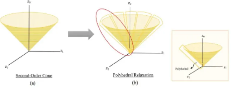
(2) 63. software, OPSEL [10], was proposed by Mullin. OPSEL is an implementation of branch and bound with an outer approximation method. Using this implementation, they successfully computed optimal solutions. However, OPSEL generates huge number of constraints in the framework of branch and bound, therefore, computing the solution by OPSEL takes long computation time. Hence, it is necessary to find a different approach to solve the problem efficiently.. The quadratic constraint in formulation (1) can be described with a second‐order cone. Through. the Cholesky factorization A=UU^{T} , the following condition can be derived:. x^{T}Ax\displaystyle \leq 2 $\theta$ N^{2}\Leftrightar ow\sum_{i}(U_{i}^{T}x_{i})^{2}\leq 2 $\theta$ N^{2}\Leftrightar ow (\sqrt{2 $\theta$}N, U^{T}) \in \mathcal{K}^{m}, where \mathcal{K}^{m} is the (m+1) ‐dimensional second‐order cone defined by. \displaystyle\mathcal{K}^{m}:=\{(v_{0},v)\in\mathb {R}+\times\mathb {R}^{r}:\sum_{k=1}^{m}v_{k}^{2}\leqv_{0}^{2}\ . Introducing a new variable y=Nx , we get MI‐SOCP formulation of our OCS problem (1): maximize. :. L_{N}^{\mathrm{T} 1. subject to. :. e^{T}y=N,. (\sqrt{2 $\theta$}N, U^{T}y) \in \mathcal{K}^{m},. y_{i}\in\{0 , 1 \} for. i=1 ,. (2). . .. , m.. However, the non‐linearity on MI‐SOCP formulation leads to heavy computation time. Therefore, we discuss approaches based on polyhedral programming relaxation, an implementation of lifted polyhedral programming (LPP) relaxation and a cone decomposition relaxation, to reduce the long computation time.. We conducted numerical experiment for the existing implementations: GENCONT and OPSEL. Since. we use CPLEX [5] can handle integer constraint on (2), we also implemented (1) on CPLEX to compare the effectiveness with our proposed methods.. The remaining of our paper is organized as follow. In Section 2 and 3, we explain our proposed ap‐ proaches based on LPP relaxation and cone decomposition, respectively. We present the numerical result for all methods in Section 4. Finally, in Section 5, we conclude our research and discuss for future studies.. 2. Lifted Polyhedral Programming Relaxation. Lifted polyhedral programming relaxation [1][4][12] is an approach to solve SOCP problems by. employing polyhedral relaxation as illustrated in Figure 1. The second‐order cone \mathcal{K}^{2} on Figure 1(\mathrm{a}) is approximated by a construction of polyhedron, to generate linear constraints since the nonlinearity of \mathcal{K}^{2} makes MI‐SOCP problems hard. More precisely, we generate many planes as in. Figure 1(b). Thus, we obtain a mixed‐integer linear programming problem as the resultant problem.
(3) 64. which can decrease the heavy computation time.. The paper [1] proposed to replace. \mathcal{K}^{m}. with a polyhedron \mathcal{K}_{$\epsilon$}^{m} using a tightness. \displaystyle \frac{\mathrm{t}\mathrm{o}1\priRcIuation me \mathrm{b}\mathrm{c}\mathrm{d}n1}{}. Sccond‐Ordcr \mathrm{C} one. (a). (b). $\epsilon$>0. so that satisfies:. \displayst le\mathrm{p},|\mathrm{y}\mathrm{h}\mathrm{e}\mathrm{M}|z\nearow^{-}\int-\swarow ’. Figure 1: Polyhedral Relaxation. \mathcal{K}^{m}\subsetneq \mathcal{K}_{ $\epsilon$}^{m}\subsetneq\{(v_{0}, v)\in \mathbb{R}+\times \mathbb{R}^{m}:| v| _{2}\leq(1+ $\epsilon$)v_{0}\}. In addition, the polyhedral relaxation \mathcal{K}_{$\epsilon$}^{m} is given as below [12]:. \mathcal{K}_{ $\epsilon$}^{m}:=\{(v_{0}, v)\in \mathbb{R}+\times \mathbb{R}^{m}:\exists($\delta$^{j})_{j=0}^{J}\in \mathbb{R}^{(T(m) } \mathrm{s}.\mathrm{t}. v_{0}=$\delta$_{1}^{J}, $\delta$_{i}^{0}=v_{i}. for. i\in\{1, \cdots , m\},. ($\delta$_{2i-1}^{j}, $\delta$_{2i}^{j}, $\delta$_{i}^{j+1}) \in \mathcal{W}_{s_{g}( $\epsilon$)} for $\delta$_{t J}^{j} =$\delta$_{\lceil t,/2\rceil}^{j+1} with. J=. \lceil\log_{2}(m)\rceil , and. for. \{t_{j}\}_{j=0}^{J}. i\in. \displaystyle \{1, \cdots ) \lf o r\frac{t_{j} {2}\rflo r\}, j\in\{0, \cdots , J-1\},. j\in\{0, \cdots , J-1\}. s.t. t_{j} is odd}. is defined recursively as follow:. \left\{ begin{ar ay}{l} t_{0}=m,&\ t_{j+1}=\lceil_{2}^{t}\lrcorner\ ceil\mathrm{f}\mathrm{o}\mathrm{r}j\in\{0,&J-1\}. \end{ar ay}\right. Using this definition, we also define T(m). =. \displaystyle \sum_{j=0}^{J}t_{j} .. In the definition of polyhedral relaxation,. \mathcal{W}_{s} expresses a polyhedron to approximate the second‐order cone \mathcal{K}^{m} defined by the following con‐ straints:.
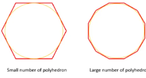
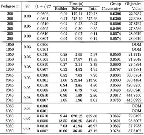
(4) 65. \mathcal{W}_{s}:=\{(v_{0}, v_{1}, v_{2})\in \mathbb{R}+\times \mathbb{R}^{2}:\exists( $\alpha$, $\beta$)\in \mathbb{R}^{2s}. v_{0}=$\alpha$_{s}\displaystyle \cos(\frac{ $\pi$}{2^{s} )+$\beta$_{s}\sin(\frac{ $\pi$}{2^{s} ) $\alpha$_{1}=v_{1}\cos( $\pi$)+v_{2}\sin( $\pi$). s.t. ,. ,. $\beta$_{1}\geq|v_{2}\cos( $\pi$)-v_{1}\sin( $\pi$)|,. $\alpha$_{i+1}=$\alpha$_{i}\displaystyle \cos(\frac{ $\pi$}{2^{i} )+$\beta$_{i}\sin(\frac{ $\pi$}{2^{i} ). ,. $\beta$_{i+1}\displaystyle \geq |$\beta$_{i}\cos(\frac{ $\pi$}{2^{i} ) -$\alpha$_{i}\sin(\frac{ $\pi$}{2^{i} )|, for. where. s. i\in\{1, s-1\}\}. is the number of the attached planes. When we use. s_{j}( $\epsilon$)=. \mathcal{W}_{s_{J}( $\epsilon$)} s_{j}( $\epsilon$) is defined with. \displayst le\lceil\frac{j+1}{2\rceil \displaystyle \lceil\log_{4}(\frac{16}{9}$\pi$^{-2}\log(1+ $\epsilon$) | j\in\{0, \cdots, J-1\}. -. for. Using the relation we can have a good approximation with small. Small number of polyhedron. $\epsilon$>0. as illustrated in Figure 2.. Large number of polyhedron. Figure 2: Effect of choosing different. $\epsilon$. We implemented this approach for different parameter values 2 $\theta$ and small $\epsilon$ > 0 using Matlab \mathrm{R}2016\mathrm{a} . We also set the duality gap 10% as the stopping criterion in CPLEX, so the accuracy of the obtained objective value is 10%. Table 1 shows the numerical results of LPP relaxation for 2 $\theta$ \{0.03 , 0.05, 0.08 \} with different (1+ $\epsilon$)2 $\theta$ . The first column in the table is the problem size m , the second is the parameter for the diversity constraint 2 $\theta$ , the third indicates $\epsilon$ to generate the LPP constraints. The $\epsilon$ is expressed by the change of group coancestry threshold from 2 $\theta$ to (1+ $\epsilon$)2 $\theta$ . For example, when we relax 2 $\theta$=0.03 to (1+ $\epsilon$)2 $\theta$=0.0301 , it means that we set $\epsilon$=0.33\times 10^{2} . The four, fifth, and six columns show the computation time to build the mathematical model, the time to solve the mathematical model and the total computation time, respectively. The last two columns show the obtained results: the group coancestry x^{T}Ax and the objective value g^{T}x. =.
(5) 66. The result on Table 1 was generated on different environment due to out of memory (OOM) while solving the problem with 2 $\theta$=0.03 . More precisely, we used a Debian Linux server on Opteron 4386. (3.10 GHz) and 128 GB memory space for the problem with 2 $\theta$=0.03 . The remaining problem was solved by a 64‐‐bit Windows 10 PC on Xeon CPU E2‐1231 (3.40 GHz) with 8 GB memory space. Table 1: LPP results for 2 $\theta$=\{0.03 , 0.05, 0.08 \}. From Table 1, we observed that LPP cannot obtain the solution for some problems with very tight 2 $\theta$ due to OOM. The utilization of the tight 2 $\theta$ makes its polyhedral relaxation (1+ $\epsilon$)2 $\theta$ generate large number of LPP constraints. Besides, LPP does not obtain optimal solution for larger $\epsilon$ . As example, the problem with (1+ $\epsilon$) =0.0306 is not optimal since the solution of group coancestry x^{T}Ax>2 $\theta$ which violates our quadratic constraint. Thus, we need to determine another tighter $\epsilon$ that will consume times. Therefore, we need another implementation to reduce the large number. of the constraints.. We combine the implementation of LPP approach with an active constraint selection method to select important constraint for our OCS problem..
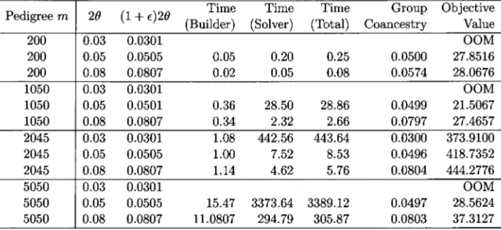
(6) 67. Definition 2.1 (Active Constraint) Let a_{i}^{T}x\leq b_{i} (i=1, \ldots,p) be inequality constraints in an optimal optimization problem with a_{i} \in \mathbb{R}^{q} and b_{i} \in \mathbb{R} (i = 1, \ldots,p) , and let x^{*} be an optimal solution of the optimization problem. We set a threshold. The inequality constraint constraint. a_{i}^{T}x\leq b_{i}. a_{i}^{T}x. \leq b_{i}. $\epsilon$>0.. is said to be active at. x^{*}. is called inactive.. if. |a_{i}^{T}x^{*}-b_{i}|. < $\epsilon$. . Otherwise, the. Algorithm 2.2 (Active constraint selection method) If an inequality constraint a_{i}^{T}x\leq b_{i} is active at some optimal solution x^{*} obtained in a preliminary experiment, we replace a_{i}^{T}x\leq b_{i} with the equality constraint. a_{i}^{T}x=b_{i}.. Using such method, we conducted preliminary experiments and found that the constraint. $\beta$_{1}\geq-v_{2}\cos( $\pi$)+v_{1}\sin( $\pi$) in the polyhedron \mathcal{W}_{s} always active at the obtained optimal solution. Therefore, we replace the constraint $\beta$_{1}\geq |v_{2}\cos( $\pi$)-v_{1}\sin( $\pi$)| by the equality $\beta$_{1}=-v_{2}\cos( $\pi$)+v_{1}\sin( $\pi$) . This replacement can reduce the number of inequalities from which we expect the reduction of computation time. Table 2 shows the computation time of the framework of LPP + active constraint. However, the. implementation of LPP relaxation combining with active selection method (LPP‐AS) requires longer computation time than LPP implementation itself. In addition, the number of problems that generated OOM is increased compared with the previous one. For example, we do not include the. result for the problem with m= {10100, 15222} since it failed to obtain the solution due to OOM. We consider that using LPP and LPP‐AS is hard depending on the chosen $\epsilon$ (see Table 1). We should determine good $\epsilon$ to obtain the optimal solution in a practical time. Therefore, we propose another implementation for solving OSC problem in the next section. Table 2: LPP‐AS results with 2 $\theta$=\{0.03 , 0.05, 0.08 \}.
(7) 68. 3. Cone Decomposition Method. The concept of cone decomposition method is similar to LPP implementation. We employ a polyhe‐ dral relaxation to solve the problem. However, the cone decomposition derives different formulation on lifted polyhedral relaxation to approximate the solution. An m‐dimensional second‐order cone can be decomposed by the following theorem. Theorem 3. 1. [ $\theta$]. Let. \displaystyle \hat{H}^{d} := \{(v_{0}, v, w)\in \mathb {R}^{(2m+1)} : v_{j}^{2}\leq \mathrm{w}_{j}v_{0}, \foral j\in\{1, \cdots , d\}, \sum_{j=1}^{d}w_{j}\leq v_{0}\}, then \mathcal{K}^{d} Proj and hence \hat{H}^{d} is a lifted reformulation of \mathcal{K}^{d} with d rotated two‐ dimensional conic quadratic constraints, one linear constraint, and d auxiliary variables. Proj(v0,v) is the orthogonal projection onto the space (v_{0}, v) variables. =. (v0,v)(\hat{H}^{d}). The utilization of the theorem makes another reformulation on our OCS (3) as follow:. g_{N}^{T}4. maximize. :. subject to. : e^{T}y=N,. z_{i}^{2}\leq w_{l}z_{0} for i=1 , . . . , m , \displaystyle \sum_{i=1}^{m}\mathrm{w}_{i}\leq z_{0}, y_{i}\in\{0 , 1 \} for. where. z_{i}=U_{i}^{T}y_{i}. for. i=1 ,. . . . , m and. i=1 ,. (3). . .. , m. z_{0}=\sqrt{2 $\theta$ N^{2}}.. Regarding the quadratic constraint in new formulation (2), we consider implementing another method to convert it into linear constraints.. Our approach is based on a Lagrange multiplier. method and outer approximation.. The following is an algorithm for an implementation of cone decomposition method based on the. theorem, the definition, an outer approximation method [3]. Algorithm 3.2 A combination of cone decomposition method with Lagrangian multiplier and Outer approximation method for OCS problem. Step 1 We compute an initial solution. formulation (3). Let. k=0.. (\hat{y}_{i}^{0},\hat{z}_{i}^{0},\hat{w}_{i}^{0}). by omitting the quadratic constraint. z_{i}^{2}. \leq w_{i}y_{0} on. Step 2. If (\hat{z}_{i}^{k})^{2} \leq \hat{w}_{i}^{k}y_{0} is violated, we compute the projection of (\hat{w}_{i}^{k}, z_{i}^{k}) onto following subproblem with the Lagrangian multiplier method.. \displaystyle \frac{1}{2}(z-\hat{y}_{i}^{k})^{2}+\frac{1}{2}(w-\hat{w}_{i}^{k})^{2}. maximize. :. subject to. : z^{2}\leq wz_{0}. Let a solution of this subproblem be. (\overline{y}_{i}^{k},\overline{z}_{i}^{k},\overline{w}_{i}^{k}) .. z_{i}^{2}. \leq. w_{i}z_{0}. by solving the.
(8) 69. Step 3. To apply an outer approximation method [3], we generate the following constraint. (w_{i}^{k_{-}\frac{i} w}k z_{i}^{k}-\overline{z}^{k})^{T}(\hat{w}_{i}^{k_{-}\frac{i} w}k \hat{z}_{i}^{k}-\overline{z}^{k})\leq0. We add the above constraint if \overline{z}_{i}^{2}-\overline{w}_{i}^{2}y_{0}>10^{-8}. Step 4 Repeat Step 2 and 3 to obtain an optimal solution if the following condition is not hold:. | \hat{z}^{2}-z <10^{-8} and | \hat{w}^{2}-w <10^{-8}. (4). Using Algorithm 3.2, we conduct numerical experiment to compare the performance of our proposed methods with the existing methods.. 4. Numerical Result. In the numerical test, we compared the performance of our proposed method with the existing method, OPSEL and GENCONT. We also compared their performances with the optimization solver CPLEX. We used the data from https: //\mathrm{d}\mathrm{o}\mathrm{i}.\mathrm{o}\mathrm{r}\mathrm{g}/10.5061/ dryad. 9\mathrm{p}\mathrm{n}5\mathrm{m} , which was generated by. \{50 , 100 \} , and the simulation POPSIM [9], for m \{200 , 1050, 2045, 5050, 10100, 15222 \}, N gap=\{1\%, 5\%\} . Moreover, we set the computation time limit to 3 hours for all methods except =. =. for LPP and LPP‐AS.. The numerical experiment was done by using a 64‐bit Windows 10 PC on Xeon CPU E3‐1231 (3.40 GHz) with 8 memory space. We implemented the proposed methods using Matlab \mathrm{R}2016\mathrm{a} . In addition, we handled the optimization problems that involve integer constraint using CPLEX.. Table 3 shows the result from a breeding selection solver GENCONT for all m except m= {10100, 15222} due to OOM. From Table 3, we observe that the number of selected candidates did not correspond to the given parameter N . This means that GENCONT failed to obtain the optimal solution since the constraint e^{T}x=N is not satisfied.. \displaystyle \frac{\mathrm{T}\mathrm{a}\mathrm{b}\mathrm{l}\mathrm{e}3:\mathrm{T}\mathrm{h}\mathrm{e}\mathrm{r}\mathrm{e}\mathrm{s}\mathrm{u}1\mathrm{t}\mathrm{f}\mathrm{r}\mathrm{o}\mathrm{m}\mathrm{G}\mathrm{E}\mathrm{N}\mathrm{C}0\mathrm{N}\mathrm{T} {N=50}. \overline{\frac{\mathrm{p}\mathrm{e}\mathrm{d}\mathrm{i}\mathrm{g}\mathrm{r}\mathrm{e}\mathrm{e}m2$\theta$g^{1}x ^{1}Ax\mathrm{T}\mathrm{i}\mathrm{m}\mathrm{e}(\mathrm{s})\#\mathrm{S}\mathrm{e}\mathrm{l}\mathrm{e}\mathrm{c}\mathrm{t}\mathrm{e}\mathrm{d}N}{20 0. 3 41 .4720. 3 403.5464} 1050. 0.0627. 25.91. 0.06270. 7.20. 81. 2045. 0.0711. 438.36. 0.07109. 111.52. 71. 5050. 0.1081. 43.44. 0.10810. 1561.43. 78. N=100. \overline{\frac{\mathrm{p}\mathrm{e}\mathrm{d}\mathrm{i}\mathrm{g}\mathrm{r}\mathrm{e}\mathrm{e}m2$\theta$g^{1}x ^{1}Ax\mathrm{T}\mathrm{i}\mathrm{m}\mathrm{e}(\mathrm{s})\#\mathrm{S}\mathrm{e}\mathrm{l}\mathrm{e}\mathrm{c}\mathrm{t}\mathrm{e}\mathrm{d}N}{20 0. 258 .890. 2580 .4893} 1050. 0.0539. 24.07. 0.0539. 4.77. 2045. 0.0628. 432.75. 0.06279. 106.48. 94. 74. 5050. 0.0994. 42.08. 0.09940. 1533.31. 81.
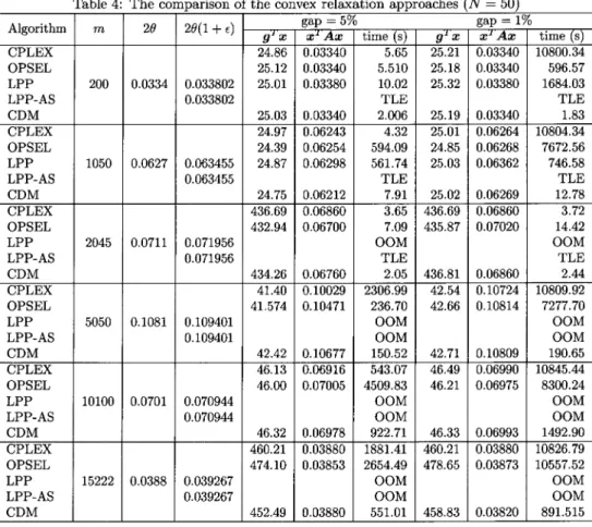
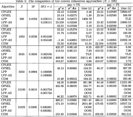
(9) 70. Table 4: The comparison of the convex relaxation approaches (N=50). Table 4 presents the result for the case. N. =. 50 .. We fixed. $\epsilon$. =. 0.006. to generate the solution. from the problem with LPP relaxation and its modification (LPP‐AS). From Table 4, LPP and LPP‐AS failed to obtain the solution due to OOM and time limit exceeded (TLE), even when the time limitation was set into 2 days. This condition is different with the result on Section 2 since we set tighter gap for the solution on here. Moreover this problem is a consequence of very tight $\epsilon$ . The chosen $\epsilon$=0.006 makes LPP cannot generate optimal solution. For example, the problem with m=200 has the value of genetic pedigree x^{T}Ax=0.00380 in which larger than 2 $\theta$=0.0334. Thus, we have to try and find another $\epsilon$ , as in Table 5. In contrast to LPP and LPP‐AS, the cone. decomposition method (CDM) takes shorter computation time than other methods. 100 . Similarly to the result on Lastly, Table 5 indicates the solution for all methods with N the previous table, LPP and LPP‐AS got no sensitive solutions for some problems due to TLE and OOM. Besides, the objective solution of LPP‐AS for Z=100 , which is equal to -1.16 , is invalid due =.
(10) 71. to time limitation. In this table, CDM gives better performance on computation time than others. Based on the above observation, CDM is the most effective method to solve OCS problem. Table 5: The comparison of the convex relaxation approaches (N=100).
(11) 72. 5. Conclusion and Future Work. In this study, we proposed the implementation of polyhedral relaxation, which is LPP, LPP‐AS, and cone decomposition methods, to optimal contribution selection of tree breeding problem. The computation time problem difficulty from OPSEL makes us consider to propose the efficiency methods for solving OCS. We compared the efficiency of our proposed implementation with the existing breeding selection software (GENCONT and OPSEL) and also with the optimization solver CPLEX. Based on the numerical result, we observed that our proposed relaxations, LPP and LPP‐AS, failed to obtain the solution for the problem with larger m due to time limitation and memory size of our environment. This condition occurred since we used very tight $\epsilon$ which will increase larger. number of constraints. Besides, very tight gaps (5% and 1%) make this method harder. Compared with LPP and LPP‐AS, GENCONT solved the problem quickly, however it only generated suboptimal solution rather than the optimal one. We also need to consider on choosing best epsilon so that LPP and LPP‐AS can guarantee the optimal solution. Therefore, we can conclude that CDM is better than other implementation in our numerical experiment since CDM can efficiently obtain the optimal solution of OCS problem. In future study, we will consider another problem of OCS that involves not only simple binary constraints but also semi‐integer constraints. References. [1] A. Ben‐Tal and A. Nemirovski. On polyhedral approximations of the second‐order cone. Math‐ ematics of Operations Research, 26(2):193-205 , 2001.. [2] C. C. Cockerham. Group inbreeding and coancestry. Genetics, 56(1):89 , 1967. [3] M. A. Duran and I. E. Grossmann. An outer‐approximation algorithm for a class of mixed‐ integer nonlinear programs. Mathematical programming, 36(3):307-339 , 1986. [4]. $\Gamma$ .. Glineur et al. Computational experiments with a linear approximation of second‐order cone. optimization. 2000.. [5] I. ILOG. Cplex optimization studio. URL: com/soflware/commerce/optimization/cplex‐optimizer, 2014.. http://www‐Ot.. ibm.. [6] M. Lubin, E. Yamangil, R. Bent, and J. P. Vielma. Extended formulations in mixed‐integer convex programming. In International Conference on Integer Programming and Combinatorial optimization, pages 102‐113. Springer, 2016.. [7] T. H. Meuwissen. Maximizing the response of selection with a predefined rate of inbreeding. Journal of animal science, 75(4):934-940 , 1997. [8] T. H. Meuwissen. Gencont: an operational tool for controlling inbreeding in selection and conservation schemes. In Proceedings of the 7th Congress on Genetics Applied to Livestock Production, pages 19‐23, 2002..
(12) 73. [9] T. J. Mullin. Using simulation to optimise tree breeding programmes in Europe: an introduction to POPSIM. Skogforsk, 2010.. [10] T. J. Mullin, J. Ahlinder, M. Yamashita, and O. Rosvall. Opsel 1.0: A computer program for optimal selection in forest tree breeding by mathematical programming. Arbetsrapport frran Skogforsk, Uppsala, Sweden, 2013.. [11] R. Pong‐Wong and J. A. Woolliams. optimisation of contribution of candidate parents to maximise genetic gain and restricting inbreeding using semidefinite programming (open access publication). Genetics Selection Evolution, 39(1):3 , 2007.. [12] J. P. Vielma, S. Ahmed, and G. L. Nemhauser. A lifted linear programming branch‐and‐bound algorithm for mixed‐integer conic quadratic programs.. INFORMS Journal on Computing,. 20(3):438-450 , 2008. [13] S. Wright. Coefficients of inbreeding and relationship. The American Naturalist, 56(645):330338, 1922.. [14] M. Yamashita, T. J. Mullin, and S. Safarina. An efficient second‐order cone programming approach for optimal selection in tree breeding. arXiv preprint arXiv:1506.04487, 2015..
(13)
図
+4

関連したドキュメント
It is a new contribution to the Mathematical Theory of Contact Mechanics, MTCM, which has seen considerable progress, especially since the beginning of this century, in
ABSTRACT: The decomposition method is applied to examples of hyperbolic, parabolic, and elliptic partlal differential equations without use of linearlzatlon techniques.. We
He thereby extended his method to the investigation of boundary value problems of couple-stress elasticity, thermoelasticity and other generalized models of an elastic
In this article we study a free boundary problem modeling the tumor growth with drug application, the mathematical model which neglect the drug application was proposed by A..
in [Notes on an Integral Inequality, JIPAM, 7(4) (2006), Art.120] and give some answers which extend the results of Boukerrioua-Guezane-Lakoud [On an open question regarding an
Although such deter- mining equations are known (see for example [23]), boundary conditions involving all polynomial coefficients of the linear operator do not seem to have been
Variational iteration method is a powerful and efficient technique in finding exact and approximate solutions for one-dimensional fractional hyperbolic partial differential equations..
This paper presents an investigation into the mechanics of this specific problem and develops an analytical approach that accounts for the effects of geometrical and material data on
