Fokas-Lenells の微分型非線形シュレーディンガー方程式の直接解法 (非線形波動研究の数理, モデリングおよび応用)

(1)

Fokas-Lenells

の微分型非線形シュレーディンガー方程式の直接解法

Direct _{method of solution for the} Fokas-Lenells

derivative nonlinear Schr\"odinger equation

山口大学大学院理工学研究科松野好雅 (Yoshimasa Matsuno)

Division of Applied Mathematical Science

Graduate School of Science

and Engineering

Yamaguchi University

E-mail address: [email protected]

Abstract

We developed

a

systematic method for obtaining soliton solutions of the

Fokas-Lenells derivative nonlinear Schr\"odingerequation ($FL$equation shortly) under

non-vanishing boundary condition. In particular,

we

deal with dark soliton solutions

with

a

plane

wave

boundary condition. We first derive the novel system ofbilinear

equations which is reduced from the $FL$ equation through

a

dependent variable

transformation and then construct the general dark $N$-soliton solution of the

sys-tem, where $N$ is anarbitrary positive integer. We then investigatethepropertiesof

the one-soliton solutions in detail, showing that both the dark and bright solitons

appear on the

nonzero

background which reduce to algebraic solitons in specific

limits. Last, the interaction process of two solitons is described.

1. Introduction

We consider the following Fokas-Lenells ($FL$) equation which can be derived from

its original version by

a

simple change of variables combined with a gauge

trans-formation:

$u_{xt}=u-2i|u|^{2}u_{x}$. (1.1)

Here, $u=u(x, t)$ is a complex-valued function of $x$ and $t$, and subscripts _$x$ and

$t$ appended to

$u$ denote partial differentiations. The known results about the $FL$

equation

are:

$\bullet$ An integrable generalization of the nonlinear Schr\"odinger equation, Fokas [1].

$\bullet$ Inverse scattering transform method under the vanishing boundary condition,

Lenells and Fokas [2].

$\bullet$ $A$ model equation for the propagation of nonlinear light pulses in monomode

optical fibers, Lenells [3].

$\bullet$ The

first

negative member of the integrable hierarchy

of the derivative nonlinear

(2)

$\bullet$

Derivation

of the bright soliton solutions,

Lenells

[4], Matsuno [5].

The purposes of the present report

are:

$\bullet$ To construct the dark $N$-soliton solution of the $FL$ equation

on

the background

of a plane wave. Explicitly, we consider the boundary condition

$uarrow\rho\exp\{i(\kappa x-\omega t+\phi^{(\pm)})\}, xarrow\pm\infty$, (1.2)

where

$\rho(>0)$

and

$\kappa$

are

realconstants representing the amplitude and wavenumber,

respectively, $\phi^{(\pm)}$

are

real phase constants and the angular frequency _{$\omega=\omega(\kappa)$}

obeys the dispersion relation $\omega=1/\kappa+2\rho^{2}.$

$\bullet$ To investigate the properties of dark soliton solutions.

This report is the summary of the paper by Matsuno [6].

2. Exact method of solution

2.1. Bilinearezation

Proposition 2.1. By

means

_of

the

dependent variable

_{tmnsformation}

$u=\rho e^{i(\kappa x-\omega t)_{\frac{g}{f’}}}$ (2.1)

with $\omega=1/\kappa+2\rho^{2}$, equation (1.1)

can

be decoupled into the following system

of

bilinear equations

_for

the $tau$

functions

$f$ and$g$

$D_{t}f\cdot f^{*}-i\rho^{2}(gg^{*}-ff^{*})=0$, (2.2)

$D_{x}D_{t}f\cdot f^{*}-i\rho^{2}D_{x}g\cdot g^{*}+i\rho^{2}D_{x}f\cdot f^{*}+2\kappa\rho^{2}(gg^{*}-ff^{*})=0$, (2.3)

$D_{x}D_{t}g\cdot f+i\kappa D_{t}g\cdot f-i\omega D_{x}g\cdot f=0$

.

(2.4)

Here, $f=f(x, t)$ and$g=g(x, t)$ are complex-valued

_{functions of}

$x$ and$t$, and the

asterisk appended to $f$ and$g$ denotes complex conjugate and the bilinear opemtors

$D_{x}$ and $D_{t}$ are

defined

by

$D_{x}^{m}D_{t}^{n}f \cdot g=(\frac{\partial}{\partial x}-\frac{\partial}{\partial x’})^{m}(\frac{\partial}{\partial t}-\frac{\partial}{\partial t’})^{n}f(x, t)g(x’, t’)|_{x’=x,t’=t}$, (2.5)

where $m$ and $n$ are nonnegative integers.

Proof. Substituting (2.1) into (1.1) and rewritingthe resultant equation in terms

of the bilinear operators, equation (1.1)

can

be rewritten

as

(3)

$- \frac{g}{f^{3}f^{*}}\{f^{*}D_{x}D_{t}f\cdot f-2\kappa\rho^{2}f^{2}f^{*}-2i\rho^{2}g^{*}(g_{x}f-gf_{x}+i\kappa fg)\}=0$. (2.6)

Inserting the identity

$f^{*}D_{x}D_{t}f\cdot f=fD_{x}D_{t}f\cdot f^{*}-2f_{x}D_{t}f\cdot f^{*}+f(D_{t}f\cdot f^{*})_{x}$, (2.7)

which can be verified by direct calculation, int$0$ the second term

on

the left-hand

side of (2.6),

one

modifies it in the form

$\frac{1}{f^{2}}(D_{x}D_{t}g\cdot f+i\kappa D_{t}g\cdot f-i\omega D_{x}g\cdot f)$

$- \frac{g}{f^{3}f^{*}}[f\{D_{x}D_{t}f\cdot f^{*}-i\rho^{2}D_{x}g\cdot g^{*}+i\rho^{2}D_{x}f\cdot f^{*}+2\kappa\rho^{2}(gg^{*}-ff^{*})\}$

$-2f_{x}\{D_{t}f\cdot f^{*}-i\rho^{2}(gg^{*}-ff^{*})\}+f\{D_{t}f\cdot f^{*}-i\rho^{2}(gg^{*}-ff^{*})\}_{x}]=0$. (2.8)

By virtue of equations $(2.2)-(2.4)$, the left-hand side of (2.8) vanishes identically.

口

It follows from (2.1) and (2.2) that

$|u|^{2}= \rho^{2}+i\frac{\partial}{\partial t}\ln\frac{f^{*}}{f}.$ (2.9)

2.2. Trilinear equation

Proposition 2.2. The trilinear equation

_for

$f$ and$g$

$f^{*} \{g_{xt}f-(f_{x}-i\kappa f)g_{t}-i(\frac{1}{\kappa}+\rho^{2})(g_{x}f-gf_{x})\}=f_{t}^{*}(g_{x}f-gf_{x}+i\kappa fg)$,

(2.10)

is a consequence

_of

the bilinear equations (2.2)-(2.4).

Proof. By direct calculation, one can show the following trilinear identity among

the tau functions $f$ and $g$:

$f^{*} \{g_{xt}f-(f_{x}-i\kappa f)g_{t}-i(\frac{1}{\kappa}+\rho^{2})(g_{x}f-gf_{x})\}-f_{t}^{*}(g_{x}f-gf_{x}+i\kappa fg)$

$=f^{*}(D_{x}D_{t}g\cdot f+i\kappa D_{t}g\cdot f-i\omega D_{x}g\cdot f)$

$- \frac{g}{2}[\{D_{t}f\cdot f^{*}-i\rho^{2}(gg^{*}-ff^{*})\}_{x}+(D_{x}D_{t}f\cdot f^{*}-i\rho^{2}D_{x}g\cdot g^{*}+i\rho^{2}D_{x}f\cdot f^{*}-2i\kappa D_{t}f\cdot f^{*})]$

$+g_{x}\{D_{t}f\cdot f^{*}-i\rho^{2}(gg^{*}-ff^{*})\}$. (2.11)

Replacing a term $2i\kappa D_{t}f\cdot f^{*}$

on

the right-hand side of (2.11) by (2.2), the

(4)

3. Dark $N$-soliton

solution

3.1. Main result

Theorem

3.1. The dark $N$-soliton solution

of

the system

of

bilinear equations

(2.2)-(2.4) is expressed by the following determinants

$f=|D|, (31a)$

$D$

$g=\tau^{1_{Z_{t}^{*}}}\rho$

$z_{1}^{T}|=|D|+\frac{1}{\rho^{2}}|_{z_{t}^{*}}^{D}$ $z_{0}^{T}|.$ $(31b)$

Here, $D$ is

an

$N\cross N$ matrix and $z$ and $z_{t}$ are $N$-component

row

vectors

defined

below and the symbol $T$ denotes the tmnspose:

$D=(d_{jk})_{1\leq j,k\leq N}, d_{jk}= \delta_{jk}+\frac{\kappa-ip_{j}}{p_{j}+p_{k}^{*}}z_{j}z_{k}^{*},$

$z_{j}= \exp(p_{j}x+\frac{\kappa\rho^{2}}{p_{j}}t+\frac{1}{p_{j}+i\kappa}\tau+\zeta_{j0}) , (3.2a)$

$Z=(z_{1}, z_{2}, \ldots, z_{N}) , z_{t}=(\frac{\kappa\rho^{2}z_{1}}{p_{1}}, \frac{\kappa\rho^{2}z_{2}}{p_{2}}, \ldots, \frac{\kappa\rho^{2}z_{N}}{p_{N}}) , (3.2b)$

where$p_{j}$

are

complex pammeters satisfying the constraints

$(p_{j}+ i\kappa)(p_{j}^{*}-i\kappa)=\frac{1+\kappa\rho^{2}}{\kappa\rho^{2}}p_{j}p_{j}^{*}, j=1,2, \ldots, N, (3.2c)$

$\zeta_{j0}(j=1,2, \ldots, N)$

are

arbitmry complex pammeters, $\delta_{jk}$ is kronecker’s delta and $\tau$ is an auxiliary variable.

3.2. Remarks

$\bullet$ The dark $N$-soliton solution is parameterized by $2N$ complex parameters

$p_{j}$ and

$\zeta_{j0}(j=1,2, \ldots, N)$

.

The parameters $p_{j}$ determine the amplitude and velocity of

the solitons whereas the parameters $\zeta_{j0}$ determine the phase of the solitons. As

opposed to the bright soliton case, however, the real and imaginary parts of$p_{j}$ are

not independent because of the constraints (3.2c).

$\bullet$ The dark $N$-soliton solution (3.1) solves the bilinear equations (2.2) and (2.3)

without the constraints (3.2c).

$\bullet$ The trilinear equation (2.10) will beproved in place ofthe bilinear equation (2.4)

where

we use

the relations

$f_{t}=(1+\kappa\rho^{2})f_{\tau}, g_{t}=(1+\kappa\rho^{2})g_{\tau}.$

(5)

4. Stability of the plane

wave

We have considered the dark solitons on the background of

a

plane

wave

$\rho e^{i(\kappa x-\omega t)}$

with $\omega=1/\kappa+2\rho^{2}$. It is important to

see

whether the background field is stable

or

not against perturbations. If unstable, then darksolitons would not exist. Here,

we

perform the linear stability analysis of the plane

wave.

Following the standard procedure, we seek a solution ofthe form

$u=(\rho+\triangle\rho)e^{i(\kappa x-\omega t+\triangle\phi)}$, (4.1)

where $\Delta\rho=\triangle\rho(x, t)$ and $\triangle\phi=\triangle\phi(x, t)$

are

small perturbations. Substituting

(4.1) into the $FL$ equation (1.1) and linearizing about the plane wave, we obtain

the system of linear PDEs for $\triangle\rho$ and $\triangle\phi$

$\triangle\rho_{xt}+\rho(\omega-2\rho^{2})\triangle\phi_{x}-\kappa\rho\triangle\phi_{t}-4\kappa\rho^{2}\triangle\rho=0, (4.2a)$

$\rho\triangle\phi_{xt}-(\omega-2\rho^{2})\triangle\rho_{x}+\kappa\Delta\rho_{t}=0. (4.2b)$ Assume the perturbations of the form $e^{i(\lambda x-\nu t)}$ with $\lambda$ real and

$v$ possibly complex

and substitute them into (4.2) to obtain

a

homogeneous linear system for $\triangle\rho$and

$\triangle\phi$

$(\lambda\nu-4\kappa\rho^{2})\triangle\rho+i\{\rho\lambda(\omega-2\rho^{2})+\kappa\rho v\}\triangle\phi=0, (4.3a)$

$-i\{(\omega-2\rho^{2})\lambda+\kappa\nu\}\triangle\rho+\rho\lambda v\triangle\phi=0. (4.3b)$

The nontrivial solution exists if $v$ satisfies the quadratic equation

$( \lambda^{2}-\kappa^{2})\nu^{2}-2(2\kappa\rho^{2}+1)\lambda\nu-\frac{\lambda^{2}}{\kappa^{2}}=0$

.

(4.4)

Solving this equation, we obtain

$\nu=\frac{\lambda}{\lambda^{2}-\kappa^{2}}[2\kappa\rho^{2}+1\pm\frac{1}{\kappa}\sqrt{\lambda^{2}+4\kappa^{3}(\kappa\rho^{2}+1)\rho^{2}}]$ (4.5)

Thus, if the condition

$\kappa(\kappa\rho^{2}+1)>0$, (4.6)

is satisfied, then $\nu$ becomes real for all values of real $\lambda$, implying that the plane

wave

is neutrally stable. It is evident that this condition always holds for $\kappa>0.$

For negative $\kappa$, on the other hand, we put $\kappa=-K$ with $K>0$ and

see

that the

stability criterion turns out to be

as

$K\rho^{2}>1.$

5. Properties of dark soliton solutions

We first parametrize the complex parameters $p_{j}$ and $\zeta_{j0}$ by the real quantities

$a_{j},$$b_{j},$$\theta_{j0}$ and

$\chi_{j0}$

as

(6)

and

introduce the

new

independent

variables

$\theta_{j}$

and

$\chi_{j}$ according to

the

relations

$\theta_{j}=a_{j}(x+c_{j}t)+\theta_{j0},$ $c_{j}= \frac{\kappa\rho^{2}}{a_{j}^{2}+b_{j}^{2}},$ $j=1,2,$ $\ldots,$

$N.$ _$(5.2a)$

$\chi_{j}=b_{j}(x-c_{j}t)+\chi_{j0}, j=1,2, \ldots, N. (5.2b)$

In terms of these variables, the variables $z_{j}$ defined by (3.2a)

are

put into the form

$z_{j}=e^{\theta_{j}+i\chi_{j}}, j=1,2, \ldots, N, (5.2c)$

after setting $\tau=0$

.

Substituting (5.1) into (3.2c), the constraints

for

$p_{j}$

can

be

rewritten

as

a

quadratic equation for $b_{j}$

$b_{j}^{2}-2\kappa^{2}\rho^{2}b_{j}+a_{j}^{2}-\kappa^{3}\rho^{2}=0, j=1,2, \ldots, N$

.

(5.3)

The solution to this equation is found to be

as

follows:

$b_{j}=(\kappa\rho)^{2}\pm\sqrt{\kappa^{3}\rho^{2}(1+\kappa\rho^{2})-a_{j}^{2}},j=1,2, \ldots, N$. (5.4)

We

can see

from the above expression that the real $b_{j}(j=1,2, \ldots, N)$ exist only

when the condition $\kappa^{3}\rho^{2}(1+\kappa\rho^{2})>0$is satisfied. This coincides with the criterion

(4.6) for the stability of the plane

wave.

Throughout the analysis,

we

assume

this

condition to

assure

the existence of soliton solutions. It is to be noted from (5.2)

and (5.3) that the parameters $a_{j}$ and $b_{j}$

are

expressed in terms of$c_{j}$

as

$a_{j}^{2}= \frac{\kappa^{2}}{4c_{j}^{2}}(c_{\max}-c_{j})(c_{j}-c_{\min})$, $b_{j}= \frac{1}{2\kappa c_{j}}(1-\kappa^{2}c_{j})$, $c_{\min}<c_{j}<c_{\max},$

$(5.5a)$

where

$c_{\max}= \frac{1}{\kappa^{2}}\{1+2\kappa\rho^{2}+2\sqrt{\kappa\rho^{2}(1+\kappa\rho^{2})}\},$

$c_{\min}= \frac{1}{\kappa^{2}}\{1+2\kappa\rho^{2}-2\sqrt{\kappa\rho^{2}(1+\kappa\rho^{2})}\}. (5.5b)$

Thus, the dark $N$-soliton solution is characterized by the $N$ velocities $c_{j}(j=$

$1,2,$ $\ldots,$$N)$ and the $2N$ real phase constants

$\theta_{j0}$ and $\chi_{j0}(j=1,2, \ldots, N)$, the total

number of which is $3N.$

5.1. One-soliton solution

The tau functions $f=f_{1}$ and $g=g_{1}$ for the one-soliton solution are given by

(7)

The one-soliton solution $u_{1}$ follows from (2.1) with (5.6), yielding

$u_{1}= \rho e^{i(\kappa x-\omega t)}1-\frac{\kappa+b_{1}}{+^{2}}\frac{a_{1}+ib_{1}}{ia_{1}a_{1}-ib_{1},e}e^{2\theta_{1}}1\frac{\kappa+b_{1}-a_{1}+ia_{1}}{2a_{1}}2\theta_{1}$ (5.7)

The above expression

can

be put into the form

$u_{1}=|u_{1}|e^{i(\kappa x-\omega t)}\exp\{i(\phi+\phi^{(+)})\}$, (5.8)

where the square of the modulus of $u_{1}$ is represented by

$|u_{1}|^{2}= \rho^{2}-\frac{2a_{1}^{2}csgn(\kappa a_{1})}{\sqrt{a_{1}^{2}+(\kappa+b_{1})^{2}}}\frac{1}{\cosh 2(\theta_{1}+\delta_{1})+\frac{(\kappa+b_{1})sgna_{1}}{\sqrt{a_{1}^{2}+(\kappa+b_{1})^{2}}}},$ $c=|c_{1}|,$ $(5.9a)$

with

$\theta_{1}=a_{1}(x+c_{1}t)+\theta_{10},$ $c_{1}= \frac{\kappa\rho^{2}}{a_{1}^{2}+b_{1}^{2}},$ $e^{4\delta_{1}}=\frac{a_{1}^{2}+(\kappa+b_{1})^{2}}{4a_{1}^{2}},$ $(5.9b)$

and the tangent of the phase $\phi$ and $\phi^{(+)}$ being given respectively by

$\tan\phi=\frac{\{a_{1}^{2}+b_{1}(\kappa+b_{1})\}\cosh 2(\theta_{1}+\delta_{1})+b_{1}sgna_{1}\sqrt{a_{1}^{2}+(\kappa+b_{1})^{2}}}{\kappa a_{1}\sinh 2(\theta_{1}+\delta_{1})},$ _$(5.10a)$

$\tan\phi^{(+)}=\frac{a_{1}^{2}+b_{1}(\kappa+b_{1})}{\kappa a_{1}}. (5.10b)$

Let us classify the one-soliton solutions in accordance with the $sign$ of $\kappa$. We

consider the two cases, i.e.,

case

1 $(\kappa>0, a_{1}\lessgtr 0)$ and case 2 $(\kappa<0, a_{1}\lessgtr 0)$

separately. For each $sign$ of $\kappa$, both dark and bright solitons arise,

as we

shall

show

now.

5.1.1. Case 1: $\kappa>0$

In this case, the velocity $c_{1}(=\kappa\rho^{2}/(a_{1}^{2}+b_{1}^{2}))$ of the soliton is positive. We then

find from (5.5) and (5.9) that

$A_{d}=\rho-\sqrt{\rho^{2}-2c_{1}\{\sqrt{a_{1}^{2}+(\kappa+b_{1})^{2}}-(\kappa+b_{1})\}}$

$= \rho-\frac{1}{\sqrt{\kappa}}|\kappa\sqrt{c}-\sqrt{1+\kappa\rho^{2}}|, a_{1}>0, c_{1}=c>0$, (5.11)

$A_{b}=\sqrt{\rho^{2}+2c_{1}\{\sqrt{a_{1}^{2}+(\kappa+b_{1})^{2}}+(\kappa+b_{1})\}}-\rho$

(8)

$c$

Figure 1. Amplitude-velocity relation for the dark soliton $A_{d}$ (solid line) and

bright soliton $A_{b}$ (broken line) for _$\rho=1$ and $\kappa=2.$

$-2 -1 0 1 2$

$x$

Figure 2. Profile of the amplitude of the dark soliton $U=|u_{1}|$ at $t=O$

.

a:

$c=c_{0}=0.75,$ $b:c=0.33,$ $c:c=0.098$. The profile

a

is

a

black soliton.

where $c\equiv|c_{1}|$ lies in the interval _{$c_{\min}<c<c_{\max}$} with $c_{\max}$ and $c_{\min}$ being given

by (5.5b). Note from (5.5a) that $\kappa+b_{1}=(1+\kappa^{2}c_{1})/(2\kappa c_{1})>0$ for $\kappa>0$ and

$c_{1}>0.$

Figure 1 plots the dependence of the amplitudes $A=A_{d}$ and $A=A_{b}$

on

the

velocity $c=|c_{1}|$ for $\rho=1$ and $\kappa=2.$

(i) Dark $\mathcal{S}oliton:a_{1}>0$

As

seen

from figure 1, the amplitude $A_{d}$ of the dark soliton becomes an increasing

function of the velocity $c$ in the interval$c_{\min}<c\leq c_{O}$ and

a

decreasing function in

the interval $c_{0}<c<c_{\max}$, where $c_{\max}$ and $c_{\min}$

are

given by (5.5b) and a critical

velocity $c_{0}$ by

$c_{0}= \frac{1+\kappa\rho^{2}}{\kappa^{2}}$. (5.13)

In the present numerical example $(\rho=1, \kappa=2),$ $c_{\min}=0.025,$ $c_{0}=0.75,$$c_{\max}=$

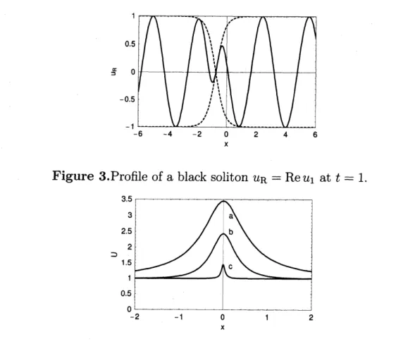
$2.47$. Figure 2 depicts the profile of $U=|u_{1}|$ at $t=0$ for three different values

of $c$, i.e.,

a:

$c=c_{0}=0.75,$ $b:c=0.33,$

$c:c=0.098$

with the parameters

(9)

$-6$ $-4$ $-2$ $0$

$\cross$

2 4

Figure 3.Profile of

a

black soliton $u_{R}={\rm Re} u_{1}$ at $t=1.$

Figure 4. Profile of the amplitude of the bright soliton $U=|u_{1}|$ at $t=0.$ a:

$c=2.47,$ $b:c=0.73,$ $c:c=0.025$. The profiles a and $c$

are

algebraic solitons.

soliton attains the maximum value $A_{d}=\rho$.

See

figure 2 $a$. It then turns out that

the intensity of the soliton center falls to zero. Such a soliton is well-known in the

field of nonlinear optics. It is sometimes called a black soliton.

Figure 3 shows the profile of $u_{R}={\rm Re}[u_{1}]$ at $t=1$ for the black soliton. The

broken line indicates $\pm|u_{1}|$ (see figure 2 a).

(ii) Bright soliton; $a_{1}<0$

Figure 4depicts theprofile of the bright soliton $U=|u_{1}|$ at $t=0$ for three different

values of $c$, i.e., a: $c=2.47,$ $b:c=0.73,$ $c:c=0.025$ with _$\rho=1$ and _$\kappa=2.$

Thefeature ofthe bright soliton differs substantiallyfrom that of the dark soliton.

To be specific, the amplitude of the bright soliton always becomes

an

increasing

function of the velocity (see figure 1). It takes the maximum value at $c=c_{\max}$

and the minimum value at $c=c_{\min}$

.

At these limiting values of the velocity, the

algebraic soliton is produced _{from the soliton of hyperbolic type.}

Indeed, if

we

put $\theta_{10}=a_{1}x_{0}-\delta_{1}$ in (5.7) and (5.9) with _{$x_{0}$} being

a

real constant

and then take the limit $a_{1}arrow-0$, we find

$x+ct+x_{0}- i\frac{2\kappa+b_{1}}{2b_{1}(\kappa+b_{1})}$

$u_{1}=\rho e^{i(\kappa x-\omega t)} (5.14a)$ $x+ct+x_{0}- i\frac{1}{2(\kappa+b_{1})},$

(10)

禾

Figure 5. Profile of an algebraic bright soliton $u_{R}={\rm Re} u_{1}$ at $t=1.$

$|u_{1}|^{2}= \rho^{2}+\frac{2\kappa c^{2}}{1+\kappa^{2_{\mathcal{C}}}}\frac{1}{(x+ct+x_{0})^{2}+(\frac{\kappa c}{1+\kappa^{2_{\mathcal{C}}}})^{2}}, (5.14b)$

where $b_{1}=(1-\kappa^{2}c)/2\kappa c$ by (4.5a) and _{$c=c_{\max}$}

or

$c_{\min}$

.

Note from (5.9b) that $b_{1}^{2}=\kappa\rho^{2}/c$ when _{$a_{1}arrow-0.$}

A representative profile of the algebraic bright soliton $U=|u_{1}|$ at $t=0$ and the

corresponding profile of$u_{R}={\rm Re} u_{1}$ at $t=1$

are

shown in figure 4

a

and figure 5,

respectively.

5.1.2. Case $2:\kappa<0$

For negative $\kappa$, the expressions of the amplitude for the dark and bright solitons

are

given respectively by

$A_{d}=\rho-\sqrt{\rho^{2}+2c_{1}\{\sqrt{a_{1}^{2}+(\kappa+b_{1})^{2}}}+(\kappa+b_{1})\}$

$= \rho-\frac{1}{\sqrt{K}}|K\sqrt{c}-\sqrt{K\prime-1}|, a_{1}<0, c_{1}=-c<0$, (5.15)

$A_{b}=\sqrt{\rho^{2}-2c_{1}\{\sqrt{a_{1}^{2}+(\kappa+b_{1})^{2}}-(\kappa+b_{1})}\}-\rho$

$= \frac{1}{\sqrt{K}}(K\sqrt{c}+\sqrt{K\rho^{2}-1})-\rho, a_{1}>0, c_{1}=-c<0$, (5.16)

where $K=-\kappa$ is a positive wavenumber and the velocity $c$ lies in the interval

$d_{\min}<c<c_{\max}’$ with

$c$

徳

$= \frac{1}{K^{2}}\{2K\rho^{2}-1+2\sqrt{K\rho^{2}(K\rho^{2}-1)}\},$

(11)

$c$

Figure 6. Amplitude-velocity relation for the dark soliton $A_{d}$ (solid line) and

bright soliton $A_{b}$ (broken line) for _$\rho=1$ and _$\kappa=-2.$

Recall that the condition $K\rho^{2}-1>0$ must be imposed to

assure

the existence of

the soliton solutions.

Figure 6 plots the dependence of the amplitudes $A=A_{d}$ and $A=A_{b}$ on the

velocity $c=|c_{1}|$ for $\rho=1$ and $\kappa=-2$. When compared with figure 1 for $\kappa>0,$

there appear several different features for $\kappa<0$. In particular, the algebraic dark

soliton would arise in the limit $carrow c_{\min}’$ since inthis limit, the amplitude $A_{d}$ tends

to a finite value. In addition, the algebraic bright soliton exists only in the limit

$carrow c_{\max}’$. We now proceed to the detailed description of the soliton solutions.

(i) Dark soliton: $a_{1}<0$

It follows from (5.5) with $\kappa=-K,$_{$c_{1}=-c$} that _{$\kappa+b_{1}=1/2Kc-K/2$}.

Since

$c_{\min}’<c<c_{\max}’$, the possible value of $\kappa+b_{1}$ is restricted by the inequality

$K[K\rho^{2}-1-\sqrt{K\rho^{2}(K\rho^{2}-1)}]<\kappa+b_{1}<K[K\rho^{2}-1+\sqrt{K\rho^{2}(K\rho^{2}-1)}]$

(5.18)

One

can see

that the upper limit of$\kappa+b_{1}$ is attainedwhen _{$c=c_{\min}’$} anditslimiting

value is positive bythe condition $K\rho^{2}>1$ whereas the lowerlimit is attained when

$c=c_{\max}’$ and is negative. In view of this fact, the algebraic dark soliton would be

produced in the limit $carrow c_{\min}’$ for which sgn$(\kappa+b_{1})>0$. Actually, taking the

limit $a_{1}arrow-0$ for the solutions (5.7) and (5.9), we find that the hyperbolic soliton

reduces to the limiting form

$x-ct+X_{0}- i\frac{-2K+b_{1}}{2b_{1}(-K+b_{1})}$

$u_{1}=\rho e^{i(-Kx-\omega t)} , (5.19a)$

$x-ct+x_{0}- i\frac{1}{2(-K+b_{1})}$

$|u_{1}|^{2}= \rho^{2}-\frac{2Kc^{2}}{1-K^{2}c}\frac{1}{(x-ct+x_{0})^{2}+(\frac{Kc}{1-K^{2}c})^{2}}, (5.19b)$

(12)

$\cross$

Figure 7. Profile of the amplitude of the dark soliton $U=|u_{1}|$ at $t=0.$

a:

$c=c_{0}=0.25,$ $b:c=0.16,$ $c:c=0.043$. The profile

a

is

a

black soliton and the

profile $c$ is

an

algebraic soliton.

Figure 8. Profile of

an

algebraic dark soliton $u_{R}={\rm Re} u_{1}$ at $t=1.$

condition $K\rho^{2}>1$, the expression $(5.19b)$ actually represents

an

algebraic dark

soliton.

Theblacksoliton appears when the velocity $c$takes

a

specific value$c=d_{0}$, where

$c_{0}’=(K\rho^{2}-1)/K^{2}$

.

(5.20)

Its profile is represented by

$|u_{1}|^{2}= \rho^{2}[1-\frac{3K\rho^{2}-4}{2(K\rho^{2}-1)}\frac{1}{\cosh 2(\theta_{1}+\delta_{1})+_{2(K\rho-1)}^{K-2}\ovalbox{\tt\small REJECT}_{2}^{2}}]$ (5.21)

It is important to notice that the inequality$d_{\min}<d_{0}<d_{\max}$ requiresthe condition

$K\rho^{2}>4/3$ for the wavenumber $K$

.

It then turns out that expression (5.21) takes

the form of

a

black soliton.

Figure 7 depicts the profile of $U=|u_{1}|$ at $t=0$ for three different values

of $c$, i.e.,

a:

$c=c_{0}’=0.25,$ $b:c=0.16,$

$c:c=0.043$

with the parameters

$\rho=1,$ $\kappa=-2,$$\theta_{10}=-\delta_{1}$ and _{$\chi_{10}=0$}

.

In this example, $d_{\min}=0.043,4=0.25$

(13)

Figure 9. Profile of the amplitude of the bright soliton $U=|u_{1}|$ at $t=0.$ a:

$c=1.46,$ $b:c=0.81,$ $c:c=0.19$. The profiles a is

an

algebraic soliton.

$-6 -4 -2 0 2 4 6$

$\cross$

Figure 10. Profile ofan algebraic bright soliton $u_{R}={\rm Re} u_{1}$ at $t=1.$

the velocity, i.e., $c=c_{\min}’$ whereas

a

black soliton arises at $c=c_{0}’$. Figure 8 shows

the profile of $u_{R}={\rm Re} u_{1}$ at $t=1$ for an algebraic dark soliton.

(ii) Bright soliton: $a_{1}>0$

Figure 9 depicts the profile of $U=|u_{1}|$ at $t=0$ for three different values of$c$, i.e.,

a: $c=1.46,$ _{$b:c=0.73,$ $c:c=0.025$} with $\rho=1$ and $\kappa=-2$. Figure 10 shows

the profile $u_{R}={\rm Re} u_{1}$ of an algebraic bright soliton at $t=1$ which corresponds to

the profile a in figure 9.

$\bullet$ Summary

i$)$ _$\kappa>0,$ $a_{1}>0$: dark soliton (no algebraic soliton)

ii) $\kappa>0,$ $a_{1}<0$: bright soliton (algebraic soliton)

iii) $\kappa<0,$ $a_{1}>0$: bright soliton (algebraic soliton)

(14)

$0$

Figure 11. The interaction of two dark solitons.

5.2.

Two-soliton solution

5.2.

1. Dark-dark solitons

The tau functions $f_{2}$

and

$g_{2}$ representing the dark two-soliton solution

are

given

by $(3.1)-(3.3)$ with $N=2$ subjected to the conditions $\kappa>0,$$a_{1}>0,$ $a_{2}>0$

.

They

read $f_{2}=1+ \frac{\kappa-ip_{1}}{p_{1}+p_{1}^{*}}z_{1}z_{1}^{*}+\frac{\kappa-ip_{2}}{p_{2}+p_{2}^{*}}z_{2^{Z_{2}^{*}}}$ $+ \frac{(\kappa-ip_{1})(\kappa-ip_{2})(p_{1}-p_{2})(p_{1}^{*}-p_{2}^{*})}{(p_{1}+p_{1}^{*})(p_{1}+p_{2}^{*})(p_{2}+p_{1}^{*})(p_{2}+p_{2}^{*})}z_{1}z_{2^{Z_{1}^{*}Z_{2}^{*}}}, (5.22a)$ $g_{2}=1- \frac{\kappa+ip_{1}^{*}p_{1}}{p_{1}+p_{i}^{*}p_{1}^{*}}z_{1}z_{i}^{*}-\frac{\kappa+ip_{2}^{*}}{p_{2}+p_{2}^{*}}\frac{p_{2}}{p_{2}^{*}}z_{2}z_{2}^{*}$ $+^{(\kappa+ip_{1}^{*})(\kappa+ip_{2}^{*})(p_{1}-p_{2})(p_{1}^{*}-p_{2}^{*})} \frac{p_{1}p_{2}}{**}z_{1}z_{2^{Z_{1}^{*}Z_{2}^{*}}}. (5.22b)$ $(p_{1}+p_{1}^{*})(p_{1}+p_{2}^{*})(p_{2}+p:)(p_{2}+p_{2}^{*})p_{1}p_{2}$

Figure 11 shows the intercaction of two dark solitons with the parameters $\rho=$

$1,$$\kappa=2,$$c_{1}=0.75,$ $c_{2}=0.24$ and $\zeta_{10}=\zeta_{20}=0$ so that from (4.14), $A_{d1}=1.0$ and

$A_{d2}=0.47.$

5. 2.2. Dark-bright solitons

Figure 12 depicts the interaction between a dark soliton and

a

bright soliton with

the parameters $\rho=1,$ $\kappa=2,$ $c_{1}=0.75,$$c_{2}=0.24$ and $\zeta_{10}=\zeta_{20}=0$, showing

that the

dark

soliton propagates faster than the bright soliton. The asymptotic

amplitudes ofthe dark and bright solitons

are

given respectively by$A_{d1}=1.0$ and

(15)

$\cup$

$0$

Figure 12. The interaction between

a

dark soliton and

a

bright soliton.

$\bullet$ Phase shift

Dark-dark solitons:

$\Delta x_{1}=\frac{1}{a_{1}}\ln|\frac{p_{1}+p_{2}^{*}}{p_{1}-p_{2}}|,$ $\Delta x_{2}=-\frac{1}{a_{2}}\ln|\frac{p_{2}+p_{1}^{*}}{p_{2}-p_{1}}|,$ _{$a_{1}>0,$} _{$a_{2}>0$}

.

(5.23)

Dark-bright

solitons:

$\Delta x_{1}=-\frac{1}{a_{1}}\ln|\frac{p_{1}+p_{2}^{*}}{p_{1}-p_{2}}|,$ $\Delta x_{2}=-\frac{1}{a_{2}}\ln|\frac{p_{2}+p_{1}^{*}}{p_{2}-p_{1}}|,$ _{$a_{1}>0,$ $a_{2}<0$}

.

(5.24)

$\Delta x_{1}>0, \Delta x_{2}<0.$

$\bullet$ Summary

i$)$ $\kappa>0,$ $a_{1}>0,$ $a_{2}>0$: dark-dark solitons

ii) $\kappa>0,$ $a_{1}>0,$ $a_{2}<0$: dark-bright solitons

iii) $\kappa>0,$ $a_{1}<0,$ $a_{2}<0$: bright-bright solitons

6. Conclusion

$\bullet$ The dark soliton solutions of the $FL$ equation have been obtained by

means

of

a

direct method.

$\bullet$ The linear stability analysis of the plane

wave

has been performed to

assure

the

(16)

$\bullet$ The

classification of the one-soliton solutons has been

done, showing

that

both

the

dark and

bright

solitons

exist

on

a

constant

background which reduce to

alge-braic solitons under certain conditions.

$\bullet$ The two-soliton solutions

can

be classified into three types, i.e., dark-dark

soli-tons, dark-bright solitons and bright-bright solitons.

Acknowledgement

This work

was

partially supported by

JSPS

KAKENHI Grant Number

22540228.

References

[1] Fokas $AS$

1995 On a

class ofphysically important integrable equations Physica

$D87145-150$

[2] Lenells $J$ and Fokas $A$ $S$

2009 On a

novel integrable generalization of the

nonlinear Schr\"odinger equation Nonlinearty 2211-27

[3] Lenells$J$ 2009Exactlysolvable model for nonlinearpulse propagationin optical

fibers Stud. Appl. Math. 123215-232

[4] Lenells $J$

2010

Dressing for

a

novel integrable generalization of the nonlinear

Schr\"odinger equation

J.

Nonlinear

Sci.

20709-722

[5] Matsuno $Y$ 2012 $A$ direct method of solution for the Fokas-Lenells derivative

nonlinear Schr\"odinger equation: I. Bright soliton solutions J. Phys. $A$: Math.

Theor.

45235202

[6] Matsuno $Y$

2012

$A$ direct method of solution for the Fokas-Lenells

derivative

nonlinear Schr\"odinger equation: II. Dark soliton solutions J. Phys. $A$: Math.