BOUNDARY
ELEMENT
APPROXIMATION OF
MINIMAL
SURFACES
AND
CONFORMAL
MAPPINGS
Takuya Tsuchiya
(
土屋卓也
)
Department of Mathematical Sciences, Faculty of Science
Ehime Unviersity (愛媛大学理学部数理科学科)
Kazuki Yoshida
(
吉田和樹
)
Graduate School ofScience and Engineering, Doctor Course
Ehime University (愛媛大学大学院理工学研究科博士課程)
Abstract. Inthis paper, boundary elementapproximationof minimal surfaces and conformal
mappings defined on the unit disk is considered. Since minimal surfaces are characterized as
stationarypointsof the Dirichlet integral in certain subsets ofafunctional space, weapproximate
the Dirichlet integral using the boundary element method and define the boundary element
minimalsurfacesasstationarypointsof the discretized Dirichlet integral. The boundary element
conformal mappingsaredefinedbythesameway. Convergence of the boundary element minimal
surfaces to the exact solutions is proved. A numerical example isgiven.
Key words. conformal mappings, minimalsurfaces, boundaryelements,variationalprinciple,
Dirichlet’s integral
AMS subject classifications. $30\mathrm{C}30,65\mathrm{E}\mathrm{o}5,65\mathrm{N}30$
1
Introduction
Let $B\subset \mathbb{R}^{2}$ be the unit disk, and
$\gamma\subset \mathbb{R}^{n}(n\geq 2)$ a closed Jordan curve. The Plateau
problem is to find
a
map $x=(x^{1}, \cdots, x^{n})\in C(\overline{B};\mathbb{R}n)\cap H^{1}(B;\mathbb{R}^{n})$ such that(1.1) $\triangle x=(\triangle x^{1}, \cdots, \triangle x^{n})=0$in $B$,
(1.2) $(X_{u_{1}}, x_{u_{2}})=|x_{u_{1}}|^{2}-|x_{u_{2}}|^{2}=0$in $B$,
(1.3) $x(\partial B)=\gamma$, and $x|_{\partial B}$ : $\partial Barrow\gamma$ is homeomorphic,
where $x_{u_{1}}:=(x_{u_{1}}^{1}, \cdots, x_{u_{1}}^{n})$ and $x_{u_{2}}:=(x_{u_{2}}^{1}, \cdots, x_{u_{2}}^{n})$
are
partial derivatives with respectto $u_{1},$ $u_{2}((u_{1}, u_{2})\in B)$, respectively, and $(\cdot, \cdot)$ and $|\cdot|$ are the usual inner product and
Euclidian
norm
in $\mathbb{R}^{n}$.If$n\geq 3$,
mean
curvaturevanishes everywhereon solutions ofthe Plateauproblem, and$x$ ofthe Plateau problem is
a
conformal mapping from $B$ to the domaindefined by theJordan curve $\gamma$ (such domains are called Jordan domains) if$x$ is orientation-preserving.
In this sense, conformal mappings are minimal surfaces in $\mathbb{R}^{2}$.
For solutions of the Plateau problem, the following variational principle has been
known (for example,
see
[3, pp.107-115], [4, Section 4.5]): Define the subset $X_{\gamma}$ of$C(\overline{B};\mathbb{R}n)\mathrm{n}H1(B;\mathbb{R}^{n})$ by
$X_{\gamma}:=\{\psi\in C(\overline{B};\mathbb{R}n)\cap H^{1}(B;\mathbb{R}^{n})|\psi(\partial B)=\gamma$and $\psi|_{\partial B}$ is $\mathrm{m}\mathrm{o}\mathrm{n}\mathrm{o}\mathrm{t}\mathrm{o}\mathrm{n}\mathrm{e}\}$,
where$\psi|_{\partial B}$ being monotone meansthat $(\psi|_{\partial B})^{-}1(p)$ is connected for any$p\in\gamma$. We denote
the Dirichlet integral (or the energy functional) on $B$ for $\varphi=(\varphi^{1}, \cdots , \varphi^{n})\in H^{1}(B;\mathbb{R}^{n})$
by
$D( \varphi):=\int_{B}|\nabla\varphi|^{2}du=\int_{B}(|\nabla\varphi|121\nabla\varphi^{n}|2)+\cdots+du$.
Then, we have that $\varphi\in X_{\gamma}$ is a solution
of
the Plateau problemif
and onlyif
$\varphi\in X_{\gamma}$ isa stationary point
of
thefunctional
$D(\varphi)$ in $X_{\gamma}$.The existence of solutions of the Plateau problem
was
proved by Douglas and Rad\’oindependently. Later on, the proof was significantly simplified by Courant (see [3] and [4]$)$. Let
$z_{1},$ $z_{2},$ $z_{3}\in\partial B$ and $\zeta_{1},$ $\zeta_{2},$ $\zeta_{3}\in\gamma$ be taken. We define $X_{\gamma}^{t\mathrm{p}}\subset X_{\gamma}$ by
$X_{\gamma}^{tp}:=\{\varphi\in X_{\gamma}|\varphi(\mathcal{Z}_{i})=\zeta i$, $i=1,2,3\}$.
Since the Dirichlet integral is invariant under conformal transformation of $B$, we have
$\inf_{y\in \mathrm{x}_{\gamma}}D(y)=\inf_{y\gamma}D(y)\in Xt\mathrm{p}$.
Theorem 1.1 (Douglas-Rad\’o-Courant)
If
$X_{\gamma}^{tp}\neq\emptyset$, then there exists at least one $x\in X_{\gamma}^{tp}$ at which the minimum valueof
the Dirichlet integral in $X_{\gamma}^{tp}$ is attained:$D(x)= \inf_{y\in^{\mathrm{x}}\gamma}Dtp(y)$.
Of
course, such $x\in X_{\gamma}^{tp}$ is a solutionof
the Plateau problem.The minimizers of the Dirichlet integral in $X_{\gamma}^{tp}$ are called the Douglas-Rad\’o
solu-tions. In
case
of$n=2$, the above existence theorem of solution ofthe Plateau problemis the Riemann mapping theorem for Jordan domains.
With the variational principle of the Plateau problem, we immediately think of the following strategy for approximatingthe Plateau problem: first, definethe discretizations
$\mathrm{S}_{\gamma,h}^{tp}$ of $X_{\gamma}^{tp}$ and $D_{h}(\varphi_{h})$ of $D(\varphi)$, respectively. Then define the discretized solutions of
the Plateau problem as stationary points of $D_{h}$ in $\mathrm{S}_{\gamma,h}^{tp}$. In [5, 6, 7, 8], the finite element
method with piecewise linear triangle elements has been used to discretized the Plateau problem. In this paper we
use
the boundary element method with piecewise linearelements to define the discretized solutions of the Plateau problem. Since we have to discritized only $\partial B$ in boundary element method, the work load for programming is much less than that of finite element method, and it seems a bit faster than FEM.
InSection 2 we definethe boundary elementminimal surfacesandconformalmappings.
In
Section 3
we prove convergence of BE solutions of the Plateau problems to the exact solutions. In Section 4 a numerical example is given.2Boundary Element Approximation
In this section, we consider
a
boundary element approximation of the Plateau problem.Let us consider the following Laplace problem with the Dirichlet boundary condition: for
given$g\in H^{1/2}(\partial B)$, find $w\in H^{1}(B)$ such
(2.1) $\triangle w=0$, in $B$, $w=g$, on $\partial B$.
With thefundamental solution$K(u, v):=-\log|u-v|/(2\pi)$fortwo-dimensional Laplacian
$\triangle$, we
obtain from (2.1) the following integral equation on $\partial B$:
(2.2) $\frac{1}{2}g(u)+\int_{\partial B}\frac{\partial K(u,v)}{\partial n_{v}}g(v)dS_{v}=\int_{\partial B}K(u, v)\frac{\partial w}{\partial n}(v)dsv$
’
for$u\in\partial B$. Solving (2.2) with the givendata
$g$on $\partial B$, we are able to obtain theNeumann
data $\partial w/\partial n$ for the solution $w\in H^{1}(B)$. In other words, we can compute the
Dirichlet-Neumann map $g\mapsto\partial w/\partial n$ associated with (2.1) by solving (2.2). By the Stokes theorem
the Dirichlet integral $D(w)$ can be computed by
$D.(w):= \int_{B}|\nabla w|^{2}du=\int_{\partial B}w\frac{\partial w}{\partial n}ds$,
if the function $w\in H^{1}(B)$ is harmonic.
In this paper we always identify $x\in C\cap H^{1/2}(\partial B;\mathbb{R}n)$ and the harmonic map $w\in$
$C(\overline{B};\mathbb{R}n)\cap H^{1}(B;\mathbb{R}^{n})$ whose Dirichlet data is
$x$ (that is, $w|_{\partial B}=x$). From the above
consideration, we
use
the equivalent form of the Dirichlet integral $D(x)$ for $x\in C\cap$$H^{1/2}(\partial B;\mathbb{R}n)$ defined by
(2.3) $D(x):= \int_{\partial B}(x^{1}\frac{\partial w^{1}}{\partial n}+\cdots+x^{n}\frac{\partial w^{n}}{\partial n})d_{S}$ ,
where the Neumann data $\partial w^{i}/\partial n$
are
obtained by solving (2.2) with$g=x$. We have the
following basic property of the Dirichlet integral:
Lemma 2.1 Let $\psi,$$\psi_{n}\in H^{1/2}(\partial B;\mathbb{R}n)$ be such that $\lim_{narrow\infty}\psi_{n}=\psi$ in $H^{1/2}(\partial B;\mathbb{R}n)$.
Then, we have $\lim_{narrow\infty}D(\psi n)=D(\psi)$.
We
are now
ready to describe the Plateau problem by the boundaryintegral equation (2.2). Let $\gamma\subset \mathbb{R}^{n}(n\geq 2)$ be a given Jordancurve.
Define the subset $X_{\gamma}\subset C\cap$$H^{1/2}(\partial B;\mathbb{R}n)$ by
$X_{\gamma}:=\{\psi\in C\mathrm{n}H1/2(\partial B;\mathbb{R}n)|\psi(\partial B)=\gamma,$ $\psi$ is $\mathrm{m}\mathrm{o}\mathrm{n}\mathrm{o}\mathrm{t}\mathrm{o}\mathrm{n}\mathrm{e}\}$.
Take arbitrary $z_{i}\in\partial B$ and $\zeta_{i}\in\gamma(i=1,2,3)$. In the
case
$n=2$,we
take those points inthe
same
orientation. Then define $X_{\gamma}^{tp}$ byLet the Dirichlet integral $D(\psi)$ for $\psi\in C\cap H^{1/2}(\partial B;\mathbb{R}2)$ be defined by (2.3). Then the
Plateau problemis:
find
$x\in X_{\gamma}^{tp}$ which is astationary pointof
the Dirichletintegral$D(\psi)$in the subset $X_{\gamma}^{tp}$.
Now it is veryclearhow we can define the boundary element solutions of the Plateau
problem.
First, we suppose that wehavea familyof triangulation $\{\triangle_{h}\}$ ofthethe l-dimensional
unit sphere $\partial B$, where $h$ stands for the maximum size of triangles (that is, intervals) in
the triangulation $\triangle_{h}$, and $harrow \mathrm{O}$. In this paper we always
assume
that$\partial B=\bigcup_{T\in\triangle_{h}}\overline{T}$
for simplicity. Let $S_{h}\subset C^{0}(\partial B)$ be the set of piecewise linear functions on each triangle. Here, the linearity is defined with respect to the arc-length parameter. We discretize$X_{\gamma}$
as
$\mathrm{S}_{\gamma,h}:=\{\psi_{h}\in(S_{h})^{n}|\psi_{h}(\partial B\cap N_{h})\subset\gamma$and $\psi_{h}|_{\partial B}$ is $d_{- \mathrm{m}\mathrm{o}}\mathrm{n}\mathrm{o}\mathrm{t}\mathrm{o}\mathrm{n}\mathrm{e}\}$ ,
where $N_{h}$ is the set of nodal points in $\triangle_{h}$, and $\psi_{h}|_{\partial B}$ being $d$-monotone
means
that theorder of nodes on $\partial B$ is preserved
on
$\gamma$ by $\psi_{h}$. Suppose that the distinct points $z_{i}\in\partial B$
and $\zeta_{i}\in\gamma(i=1,2,3)$ are taken as above. We
assume
that $z_{i}\in\partial B$ are nodal points of$\triangle_{h}$ for each $h>0$. Then we define
$\mathrm{S}_{\gamma,h}^{tp}:=\{\psi_{h}\in \mathrm{S}_{\gamma,h}|\psi_{h}(Z_{i})=\zeta i,$ $i=1,2,3\}$.
For $\psi_{h}\in(S_{h})^{n}$ we compute the discretized Dirichlet integral $D_{h}(\psi_{h})$ by the
$\mathrm{f}\mathrm{o}\mathrm{l}1_{0}\mathrm{W}\mathrm{i}\mathrm{n}.\mathrm{g}$
manner.
First, we compute the solution of the Laplace equation$\triangle w=0$ in $B$, $w=\psi_{h}$ on $\partial B$,
by certain boundary element method on the space $(S_{h})^{n}$, and obtain its approximated
Neumann data $(\partial w/\partial n)_{h}=((\partial w^{1}/\partial n)_{h}, \cdots, (\partial w^{n}/\partial n)_{h})\in(S_{h})^{n}$. Then, $D_{h}(\psi_{h})$ is
de-fined by
(2.4) $D_{h}( \psi_{h}):=\int_{\partial B}(\psi_{h}^{1}(\frac{\partial w^{1}}{\partial n})_{h}+\cdots+\psi^{n}h(\frac{\partial w^{n}}{\partial n})_{h})ds$.
A stationary point $x_{h}\in \mathrm{S}_{\gamma,h}^{tp}$ of $D_{h}(\psi_{h})$ in the subset $\mathrm{S}_{\gamma,h}^{tp}$ is called a boundary
ele-ment minimal surface. In the
case
$n=2$ it is calleda boundary element conformalmapping. In particular, the minimizer $x_{h}$ of the discretized Dirichlet integral$D_{h}$ in $\mathrm{S}_{\gamma,h}^{tp}$
is called the boundary element Douglas-Rad\’o solution.
3
Convergence
of BE
Minimal Surfaces
In this section
we
considerconvergence
of the boundary element minimal surfaces. To dothis we require the following reasonable assumption:
Assumption 3.1 There exists a nonnegative
function
$g(h)$for
$h>0$ such that$\lim_{harrow 0}g(h)=0$ and,
for
sufficiently small $h>0$,(3.1) $(1-g(h))D_{h}(\psi_{h})\leq D(\psi_{h})\leq(1+g(h))D_{h}(\psi_{h})$,
for
any $\psi_{h}\in(S_{h})^{n}$, where the Dirichlet integrals $D$ and $D_{h}$are
defined
by (2.3) and (2.4),In Assumption 3.1 we require that the boundary element method we use can attain
sufficient accuracy so that the discretized Dirichlet integral $D_{h}$ is a good approximation
ofthe exact Dirichlet integral $D$. This is the only assumption we need for the boundary
element method in this paper.
Lemma 3.2 Suppose that Assumption 3.1 holds. Let $\{\psi_{h}\in(S_{h})^{n}\}$ be a sequence such
that $D_{h}(\psi_{h})\leq M$ with some positive constant M. Suppose that $\{\psi_{h}\}$ converges uniformly
to a continuous map $\psi\in C(\partial B;\mathbb{R}^{n})$. Then we have $\psi\in H^{1/2}(\partial B;\mathbb{R}n)$ and (3.2) $D( \psi)\leq\lim_{harrow}\inf_{0}Dh(\psi_{h})$.
Proof.
Let $f,$ $f_{h}$ be harmonic maps with $f=\psi,$ $f_{h}=\psi_{h}$ on $\partial B$, respectively. Since $\psi_{h}$converges uniformly to$\psi$, and in viewofwell-known lower semicontinuity of the Dirichlet
integral, we have $D( \psi)=D(f)\leq\lim\inf_{harrow 0^{D(f_{h}}})=\lim\inf_{harrow 0^{D}}(\psi_{h})\leq M$. Hence,
$f\in H^{1}(B;\mathbb{R}^{n})$ and $f|_{\partial B}=\psi\in H^{1/2}(\partial B;\mathbb{R}n)$. By (3.1), we obtain (3.2). $\square$
The following lemmais on the relative compactness ofbounded subsets of$\mathrm{S}_{\gamma,h}^{tp}$, which
is the most crucial in our convergence analysis.
Lemma 3.3 ([7], Lemma6) Suppose that Assumption 3.1 holds and the given Jordan
curve is
rectifiable.
Take a sequence $\{\psi h\in \mathrm{S}_{\gamma,h}^{tp}\}$.
Weassume
that $D_{h}(\psi_{h})$ are uniformlybounded. Then, there exists a subsequence $\{\psi_{\mathrm{t}_{i}}\}$ such that $\psi_{h_{i}}$ converges uniformly to a
continuous map $\psi\in C\cap H^{1/2}(\partial B;\mathbb{R}n)$ on $\partial B$. Moreover, $\psi\in X_{\gamma}^{tp}$.
Theorem 3.4 Suppose that Assumption 3.1 holds and the given Jordan curve $\gamma$ is
rec-tifiable.
Let $\{x_{h}\in \mathrm{s}_{\gamma,h}^{t}\mathrm{P}\}$ be a sequenceof
the boundary element Douglas-Rad\’o solutions.Then there exists a subsequence $\{x_{h_{i}}\}$ which converges to one
of
the exact Douglas-Rad6solutions $x\in X_{\gamma}^{tp}$ in the following sense:
(3.3) $\lim_{h_{i^{arrow}}0}||x-Xh_{i}||_{C(\partial B\mathbb{R})};n=0$,
(3.4) $\lim_{h_{i}arrow 0}||_{X}-xh_{i}||H1/2(\partial B;\mathbb{R}^{n})=0$.
Proof.
Since $\mathrm{S}_{\gamma,h}^{tp}$ are bounded closed subsets in a finite dimensional vector spaces, it isobvious that the boundary element Douglas-Rad\’o solutions exist in each $\mathrm{S}_{\gamma,h}^{tp}$.
Let $y\in X_{\gamma}^{tp}$ be one of the Douglas-Rad\’o solutions. Let $\Pi_{h}$ : $C(\partial B;\mathbb{R}n)arrow(S_{h})^{n}$ be the usual interpolant projection (see [2]), that is, $\Pi_{h}y\in(S_{h})^{n}$ is defined so that
$\Pi_{hy}(u_{j})=y(u_{j})$ for nodal points $u_{j}$ of $\triangle_{h}$. It follows from Lemma 2.1 and (3.1) that $\lim_{harrow 0}D_{h}(\Pi_{h}y)=D(y)$.
Since $D_{h}(x_{h})\leq D_{h}(\Pi_{h}y),$ $\{D_{h}(X_{h})\}$ is uniformlybounded. Thus, byLemma3.3, there
exists asubsequence $\{x_{h_{i}}\}$ which converges uniformly to a continuous map $x\in X_{\gamma}^{tp}$. By
Lemma3.2
we
obtain(3.5) $D(x) \leq\lim_{h_{i}arrow}\inf_{0}Dh_{i}(x_{h}i)\leq\lim_{h_{i}arrow 0}Dhi(\Pi hiy)=D(y)$.
Now, let $w,$ $w_{h_{i}}\in H^{1}(B;\mathbb{R}^{n})$ be harmonic maps with $w=x,$ $w_{h_{i}}=x_{h_{i}}$ on $\partial B$,
re-spectively.Since
$||w_{h_{i}}||_{H^{1}()}B;\mathbb{R}^{n}$ are uniformly bounded, $\{w_{h_{i}}\}$ has a weakly convergentsubsequence. We know that, by the maximum principle of harmonic maps, $\{w_{h_{i}}\}$
con-verges to $w$ uniformly on $\overline{B}$
. Therefore, $w_{h_{i}}$ converges to $w$ weakly in $H^{1}(B;\mathbb{R}^{n})$. Also
we have
(3.6) $\lim_{h_{i^{arrow}}0}||w-Wh_{i}||_{L^{2}(\cdot)}B,\mathbb{R}^{n}=0$.
On the other hand, we have $D(x)=D(w)$ and $D(x_{h_{i}})=D(w_{h_{i}})$. With (3.1) and (3.5)
we
get(3.7) $\lim_{h_{i}arrow 0}|w_{h_{i}}|2H1(B;\mathbb{R}^{n})=\lim_{0h_{i}arrow}D(w_{h_{i}})=D(w)=|w|_{H^{1}()}2B;\mathbb{R}^{n}$.
Combining (3.6) and (3.7) we obtain
$\lim_{h_{i}arrow 0}||w-wh_{i}||H1(B;\mathbb{R}^{n})=\lim_{h_{i}arrow 0}||w|_{\partial B}-w_{h_{i}}|\partial B||_{H(\partial B}1/2\mathbb{R}n;)=0$.
Therefore (3.4) is proved.
If the Douglas-Rad\’o solution is unique, the limit of convergent subsequence of $\{x_{h}\}$
is unique. Hence $x_{h}$ converges to the unique Douglas-Rad\’o solution in the sense of (3.3)
and (3.4). $\square$
Corollary 3.5 Suppose that Assumption 3.1 holds and the given Jordan curve $\gamma$ is
rec-tifiable.
Let $n=2$ and $\{x_{h}\in \mathrm{S}_{\gamma,h}^{tp}\}$ the sequenceof
the boundary elementconformal
mappings. Then $\{x_{h}\}$ converges to the unique
conformal
mapping $x\in X_{\gamma}^{tp}$ in the senseof
(3.3) and (3.4).A map$x\in X_{\gamma}^{tp}$issaid to bean isolated stable minimal
surface
ifthere existsaconstant$\delta$ such that
$0<||x-y||c(\partial B;\mathbb{R}^{n})<\delta$ implies $D(x)<D(y)$ for $y\in X_{\gamma}^{tp}$.
Theorem 3.6 Suppose that Assumption 3.1 holds and the given Jordan curve $\gamma$ is
rec-tifiable.
Let $x\in X_{\gamma}^{tp}$ be an isolated stable minimalsurface.
Then there exists a sequence$\{x_{h}\in \mathrm{S}_{\gamma)h}^{tp}\}$
of
stable boundary element minimalsurfaces
which converges to $x$ in the senseof
(3.3) and (3.4).Proof.
As in the proof on Theorem 3.4, let $\Pi_{h}$ : $C(\partial B;\mathbb{R}n)arrow(S_{h})^{n}$ be the interpolantprojection. We define $\delta$-neighborhoods of $\Pi_{h}x$ by
$U_{h}^{\delta}(\Pi_{h^{X)}}:=\{\psi_{h}\in \mathrm{s}^{tp}\gamma,h|||\psi_{h}-\square _{h}x||c(\partial B;\mathbb{R}^{n})\leq\delta\}$ .
Since $U_{h}^{\delta}(\Pi_{h}x)$ is
a
bounded closed set in finite-dimensional Euclidean space, there exists$x_{h}\in \mathrm{S}_{\gamma,h}^{tp}$ such that $D_{h}(x_{h})$ attains the minimum value of $D_{h}$ in $U_{h}^{\delta}(\Pi_{h}x)$. By (3.5)
$\{D_{h}(X_{h})\}$ is uniformly bounded. Hence there exists a subsequence $\{x_{h_{i}}\}\vee$ which converges
For arbitrary $\epsilon>0$ we take sufficiently small $h_{i}>0$
so
that $||x-\Pi_{h_{i}}x||_{c}(\partial B;\mathbb{R}n)<\epsilon/2$ and $||\psi-X_{h_{i}}||_{C(\partial B\mathbb{R})};n<\epsilon/2$. We then obtain$||\psi-X||C(\partial B;\mathbb{R}^{n})<\in+||\Pi_{h}ix-X_{h_{i}}||_{C()}\partial B;\mathbb{R}^{n}\leq\in+\delta$.
Hence we show that $||\psi-x||C(\partial B;\mathbb{R}^{n})\leq\delta$ and, by the definition, $D(\psi)\geq D(x)$. On the other hand, from the lower-semicontinuity of the Dirichlet integral and (3.5) we have
$D(\psi)\leq D(x)$. Thus we conclude that $D(\psi)=D(x)$, and, again by the assumption,
$x=\psi$. By the exactly same way as in the proof of of Theorem 3.4 we can show that $x_{h}$
converges to $x$ in the
sense
of (3.3) and (3.4). Because of the convergence we have justproved, we now know that, for sufficiently small $h>0,$ $x_{h}$ are inner points in $U_{h}^{\delta}(\Pi_{h}x)$.
Hence they are boundary element minimal surfaces. $\square$
4
A
Numerical Example
In this section we give a numerical example. Let $n=2$ and $\gamma=(\gamma_{1}, \gamma_{2})\subset \mathbb{R}^{2}$ defined by $\gamma_{1}(\theta):=(1+C\cos 3\theta)\cos\theta$, $\gamma_{2}(\theta):=(1+C\sin 3\theta)\sin\theta$,
for $\theta\in[0,2\pi]$, where $C$ is a constant. Let $z_{i}:=\exp(\sqrt{-1}\theta_{i}),$ $\zeta_{i}:=\gamma(\theta_{i})$, and $\theta_{i}$ $:=$
$2(i-1)\pi/3,$ $(i=1,2,3)$. Let $\Omega$ be the Jordan domain bounded by
$\gamma$. We compute
conformal mapping $x\in X_{\gamma}^{tp}$ from $B$ to $\Omega$ with $x(z_{i})=\zeta_{i}(i=1,2,3)$. We do so by the
finite element methods ([5, 6, 7, 8]) and the boundary element methods, and compare the results. The image of the finite element conformal mappings may be found in [5].
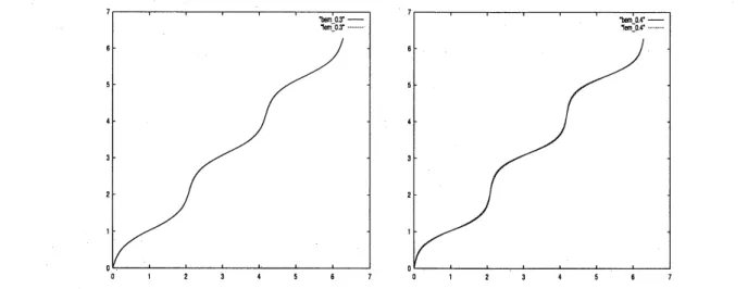
In Figure 4.1,4.2 we show the graphsof the function $y_{h}$ : $[0,2_{T}]arrow[0,2\pi]$ with various
$C$. The boundary element and finite element conformal mappings $x_{h}$ : $\partial Barrow\gamma$ are
obtained as $x_{h}(\theta):=\Pi_{h}\gamma(y_{h}(\theta))$. For both methods the number of nodes on $\partial B$ is 120. We notice that the boundary element and finite element conformal mappings are almost identical when $C\leq 0.4$. However, there are some gaps between them with $C>0.4$.
Probably, it is because boundary nodes tend to gather the narrowpart of$\gamma$, andtherefore
the accuracy of the approximation becomes inferior on the rest of the boundary in one of
(or both of) the methods.
Figure 4.2: Comparison of FE and BE conformal mappings. $C=0.45$ and $C=0.5$
.
References
[1] G. Chen, J. Zhou, Boundary Element Methods, Academic, 1992
[2] P.G. Ciarlet, The Finite Element Methods for Elliptic Problems, North Holland, 1978
[3] R. Courant, Dirichlet’s Principle, Conformal Mappings, and Minimal Surfaces, In-terscience 1950, reprint by Springer 1977
[4] U. Dierkes, S. Hildebrandt, A. K\"uster, O. Wohlrab, Minimal Surfaces I, Springer,
1992
[5] T. Tsuchiya, On two methods for approximating minimal surfaces in parametric form, Math. Comp.
46
(1986) 517-529.[6] T. Tsuchiya, Discrete solution of the Plateau problem and its convergence, Math. Comp. 49 (1987) 157-165.
[7] T. Tsuchiya, A note
on
discrete solutions of the Plateau problem. Math. Comp.54
(1990) 131-138.