A Numerical Approximation Method for a Non-local Operator Applied to Radiation Problem (Discretization Methods and Numerical Algorithms for Differential Equations)

(1)

A

Numerical

Approximation Method for aNon-local

Operator Applied

to

Radiation Problem

Haniffa M. NASIR(ハニファモハメドナシル), Universityof Peradeniya1

KAKO,Takashi(加古孝), TheUniversityofElectrO-Communications (電気通信大学)2)

Abstract : Inthefinite element approximationof the exterior Helmholtzproblem, wepropose

an

approximationmethod to implement the$\mathrm{D}\mathrm{t}\mathrm{N}$ mappingformulatedas apseud0-differentialoperator

on acomputational artificial boundary. The method is then combined with the fictitious domain

method. Our method directlygivesan approximation matrix for the sesqui-linearform for the $\mathrm{D}\mathrm{t}\mathrm{N}$

mapping. The eigenvalues of the approximation matrix is simplified to aclosed form and can be

computed efficiently by using acontinued fraction formula. Solution outside the computational

domain and thefar-field solutioncan also becomputedefficiently by expressing them asoperations

ofpseud0-differential operators. Aninner artificial $\mathrm{D}\mathrm{t}\mathrm{N}$ boundaryconditionis also implemented by

our

method. We prove the convergenceof the solution ofourmethod and compare the performance

with the standard finiteelement approximation based on the Fourier series expansion ofthe $\mathrm{D}\mathrm{t}\mathrm{N}$

operator. The efficiency ofour method is demonstrated through numerical examples.

1Introduction

We consider the following tw0-dimensionalexterior Helmholtzproblem:

$-\Delta u-k^{2}u$ _$=$ ₀ _in $\Omega=\mathbb{R}^{2}\backslash O$, (1a) $\frac{\partial u}{\partial n}$

$=$ $- \frac{\partial u^{\mathrm{i}\mathrm{n}\mathrm{c}}}{\partial n}$ on$\partial\Omega$, (1b)

$\lim_{rarrow\infty}\sqrt{r}(\frac{\partial u}{\partial r}-\mathrm{i}ku)$ $=$ 0, (1c)

where 0is the interior of the complement of abounded region $O$ in $\mathrm{R}^{2}$ with smooth boundary

an

on which the Neumann boundary condition (1b) is imposed and (1c) is the Sommerfeld radiation

condition at infinity.

The equationcanbe used to simulate thescatteringphenomenaoftime-harmonicelectromagnetic

or acousticwaveby anobstacle $O$which is sometimes called ascatterer. Here, $u^{\mathrm{i}\mathrm{n}\mathrm{c}}(\mathrm{x})=\mathrm{e}^{\mathrm{i}\mathrm{k}.\mathrm{x}}$is the

time-harmonic incident planewave whose direction ofpropagation is given by the vector $\mathrm{k}$, and

$\mathrm{n}$

is the outward unit normalon the scatterer (see Fig. 1).

$\ovalbox{\tt\small REJECT}^{\nearrow\nearrow\nearrow}\Omega$

.

Figure 1: Obstacle and artificial boundary

In orderto solve the exteriorHelmholtzproblems numerically, it is

acommon

practiceto intro

duce an artificialboundary to limit theareaof computation and to prescribean artificialboundary

condition on this boundary. The boundary condition is expected to “absorb” the outgoingwaves

and to exclude any incomingwaves. Various artificial boundary conditions have been proposed in

the literature for this purpose (see Givoli [6], Ihlenburg [8] and the references therein). The

artifi-cialboundary condition that gives the solution to (1) is given by the Dirichlet toNeumann $(\mathrm{D}\mathrm{t}\mathrm{N})$

mapping.

Universityof Peradeniya, SriLanka. Email: nasirhm@fedu.uec.ac.jp

$2\mathrm{T}\mathrm{h}\mathrm{e}$University of

ElectrO-Communications, Chofu, Japan. Email: kako@im.uec.ac.jp

数理解析研究所講究録 1265 巻 2002 年 173-183

(2)

In thefinite element approximation of the problem, theimplementation of the $\mathrm{D}\mathrm{t}\mathrm{N}$ mappingor

its approximations has been asubject of interest by many authors (see, for example, Kako [9], Liu

[13], Liu and Kako [14] and the referencestherein). Asfor the

case

of using theexact$\mathrm{D}\mathrm{t}\mathrm{N}$maPPing,

MacCamy and Marin [16] used an integral representationofthe $\mathrm{D}\mathrm{t}\mathrm{N}$ mapping and obtain itsfinite

element matrix by explicitly solving

some

auxiliary integral equations. Keller and Givoli [10] used

the Fourier series representation of the$\mathrm{D}\mathrm{t}\mathrm{N}$ mapping andusethe standard finite element technique

toobtain the matrix in

an

infinite series form (see also Ernst [4] and Heikkolaet al. [7]).

Inthispaper,we propose anapproximationmethodtoimplementthe$\mathrm{D}\mathrm{t}\mathrm{N}$mapping by expressing

it in aform of pseudo differential operator. The finite element approximation corresponding to the

sesqui-linear form of the pseudo differential operator is given by amatrix which

we

call amixed

type approximation matrix. This matrix is obtained by replacing the argument of the function

in the pseudodifferential operator, which in this

case

is the Laplacian

on

the unit circle, by its

finite element matrix. This gives amatrix in aclosed form which

can

be efficiently computed by a

continued fraction without

use

of the Hankel function and its derivative. The computational cost

for the boundary condition in this method is$O(n_{\theta})$ where$n\theta$ isthenumber of partitions in angular

direction.

When theoriginof the polar-coordinatesystemisoutside the obstacledomain,

one can

consider

an inner artificial boundary that excludes the origin from the computational domain and another

$\mathrm{D}\mathrm{t}\mathrm{N}$ boundary condition is imposed

on

the inner artificial boundary which is also treated by

our

method.

Thesolution outside thecomputational domain and the far-fieldpattern

are

expressed inclosed

formsbyusingpseudodifferentialoperatorsandourpreviousmethodcanalsobeappliedtocompute

the quantities.

We consider the fictitious domain method to form the linear equations and use the Krylov

subspace iterative method to solve the linear system (Kuznetsovet al. [12], Heikkola et al. [7]).

The rest of the paper is organized

as

follows. In Section 2,

we

review the artificial boundary

condition and its standard finite element approximation. In Section 3, we introduce amixed tyPe

method for the artificial boundary and its application in fictitious domain method. In Section 4,

we consider the application of the mixed tyPe method for the solution outside the computational

domain and the far-field pattern. InSection5,

we

provetheconvergence ofthesolutions. Wepresent

the results of numerical tests in Section 6and makesome concluding remarks inSection 7.

2Artificial boundaries

and artificial

boundary

conditions

For the numerical treatmentof theproblem (1),the unbounded domain0istruncatedbyanartificial

boundary, denotedby$\Gamma_{R}$,andanartificial boundary conditionisintroduced. The artificial boundary

is acircle of radius $R$ and we denote by$B_{R}$ the circular domain ofradius $R$ bounded by $\Gamma_{R}$

.

The

approximate boundary value problem is then given by

$-\Delta u-k^{2}u$ $=$ 0 in $\Omega_{R}\equiv\Omega\cap B_{R}$, (2a)

$\frac{\partial u}{\partial n}$

$=$ $- \frac{\partial u^{\mathrm{i}\mathrm{n}\mathrm{c}}}{\partial n}$

on $\partial\Omega$, (2b)

$\frac{\partial u}{\partial r}$

$=$ $-Mu$

on

$\Gamma_{R}$, (2c)

where M isthe DtN mapping which weregard

as

apseudodifferentialoperator

as

afunctionof the

Laplacian operator $D^{2}:=-\partial^{2}/\partial\theta^{2}$ and is given by

$M(D^{2})u(R,\theta)$ $\equiv$ $- \frac{k}{2\pi}\sum_{n=-\infty}^{\infty}\frac{H^{(1)’}(kRn)}{H^{(1)}(kRn)}\int_{0}^{2\pi}u(R, \phi)\mathrm{e}^{\mathrm{i}n(\theta-\phi)}d\phi$ (3)

$=$ $-k \frac{H^{(1)’}(kR\sqrt{D^{2}})}{H^{(1)}(kR_{j}\sqrt{D^{2}})}u(R,\theta)$, (4)

(3)

where wedenote by $H^{(1)}(x;\nu)$ the Hankel function ofthe first kind of order$\nu$

.

The basic definition

ofpseud0-differential operatorcan be found, for example, in Nirenberg [18] and Taylor [19].

2.1 Weak

formulation

and

FEM

Let $V\equiv H^{1}(\Omega_{R})$ where $H^{s}(\Omega_{R})$ is the Sobolev space of order $s\in \mathrm{R}$ in $\Omega_{R}$ and

$\gamma$ : $H^{1}(\Omega_{R})arrow$

$H^{1/2}(\Gamma_{R})$ be the $\mathrm{t}\mathrm{r}\mathrm{a}\mathrm{c}\mathrm{e}$operator. Then, the weak

formulation of the boundary valueproblem (2) is:

Find $u\in V$ suchthat

$a(u, v)+\langle\gamma u, \gamma v\rangle_{M}=(\partial u^{\mathrm{i}\mathrm{n}\mathrm{c}}/\partial n, v)_{\partial\Omega}$ $\forall v\in V$, (5)

where the sesqui-linearforms$a(\cdot$,$\cdot$$)$, $\langle\cdot$,$\cdot\rangle_{M}$ and $(\cdot$,$\cdot)_{\partial\Omega}$ respectively

are

$a(u, v)$ $=$ $\int_{\Omega_{R}}(\frac{\partial u}{\partial r}\frac{\partial\overline{v}}{\partial r}+\frac{1}{r^{2}}\frac{\partial u}{\partial\theta}\frac{\partial\overline{v}}{\partial\theta}-k^{2}u\overline{v})$ rdrdfl, $u$,$v\in H^{1}(\Omega_{R})$,

$\langle p, q\rangle_{M}$ $=$ $\int_{0}^{2\pi}(Mp)(\theta)\overline{q}(\theta)Rd\theta$,

$p$,$q\in H^{1/2}(\Gamma_{R})$,

and $(f, g)_{\partial\Omega}$ $=$ $\int_{\partial\Omega}f\overline{g}d\sigma$, $f$,$g\in L^{2}(\partial\Omega)$

.

Now, based on the element partitioning ofthe computational domain described in Subsection 3.2,

we form afinite dimensional subspace $V_{h}$ of $V$

.

The finite element approximate problem is then

given by: Find $u_{h}\in V_{h}$ such that

$a(u_{h}, v_{h})+\langle\gamma u_{h}, \gamma v_{h}\rangle_{M}=(\partial u^{\mathrm{i}\mathrm{n}\mathrm{c}}/\partial n, \mathrm{v})\mathrm{d}\mathrm{Q}$, $\forall v_{h}\in V_{h}$

.

(6)

2.2 FEM matrix of DtN mapping

by

the

Fourier

mode representation

The finite element approximation matrix corresponding to the $\mathrm{D}\mathrm{t}\mathrm{N}$ mappings given in the form of

(3) has been obtainedby several authors (e.g., Ernst [4]).

According to the finite element partitioning of $\Omega_{R}$, the artificial boundary $\Gamma_{R}$ is discretized by

auniform partitioning with $n_{\theta}$ nodes and an equal number of intervals. We use piecewise linear

continuous functions $\{\phi_{i}\}_{i=0}^{n_{\theta}-1}$ as the basis for the finite element approximation. The sesqui-linear

form corresponding to the$\mathrm{D}\mathrm{t}\mathrm{N}$ mappingis represented in terms of the Fourier modes

as

$\langle\gamma u_{h}, \gamma v_{h}\rangle_{M}$ $=$ $\sum_{n=-\infty}^{\infty}RM(n^{2})\overline{\gamma u}_{h,n}\overline{\overline{\gamma v}_{h,n}}$ (7)

where$\hat{p}_{h,n}$ is the Fourier coefficient of

$p_{h}$ given by$\hat{p}_{h,n}=\frac{1}{\sqrt{2\pi}}\int_{0}^{2\pi}p_{h}(\phi)\mathrm{e}^{-\mathrm{i}n\phi}d\phi$

.

We express$p_{h}= \sum_{j=0}^{n_{\theta}1}\overline{p}_{h,\mathrm{j}}\phi_{j}(\theta)$and set $[\tilde{\mathrm{p}}_{h}]:=[\tilde{p}_{h,0},\tilde{p}_{h,1}, \cdots,\tilde{p}_{h,n_{\theta}-1}]^{T}$

.

By perfo rming the

integration, we get $\overline{\gamma u}_{h,n}=\mu_{n}Q_{h,n}[\overline{\gamma u}_{h}]$, where $\mu_{0}=\sqrt{h_{\theta}}$, _{$\mu_{n}=2(1-\cos nh_{\theta})/(n^{2}h_{\theta}^{3/2})$} for $n\neq 0$, $Q_{h,n}=[1,\mathrm{e}^{\mathrm{i}2\pi n/n_{\theta}}, \cdots, \mathrm{e}^{\mathrm{i}2\pi n(n_{\theta}-1)/n_{\theta}}]/\sqrt{n_{\theta}}$and $h_{\theta}=2\pi/n_{\theta}$

.

Clearly, $Q_{h,j}=Q_{h,\downarrow n_{\theta}+j}$ for

$0\leq j<n_{\theta}$,$l\in \mathbb{Z}$. Substituting$\overline{\gamma u}_{h,n}$ and$\overline{\gamma v}_{h,n}$ in (7), we have

$\langle\gamma u_{h},\gamma v_{h}\rangle_{M}$ _$=$ $\sum_{n=-\infty}^{\infty}\overline{[\overline{\gamma v}_{h}]^{T}Q_{h,n}^{T}}RM(n^{2})\mu_{n}^{2}Q_{h,n}[\overline{\gamma u}_{h}]$

$=$ $\sum_{j=0}^{n_{\theta}-1}\overline{[\overline{\gamma v}_{h}]^{T}Q_{h,j}^{T}}\sum_{t=-\infty}^{\infty}RM((ln_{\theta}+j)^{2})\mu_{ln_{\theta}+j}^{2}Q_{h,j}[\overline{\gamma u}_{h}]$

$=$: $(\mathrm{M}_{h}^{\mathrm{s}\mathrm{t}\mathrm{d}}[\overline{\gamma u}_{h}], [\overline{\gamma v}_{h}])_{\mathbb{C}^{n_{\theta}}}$, (8)

where $\mathrm{M}_{h}^{\mathrm{s}\mathrm{t}\mathrm{d}}=Q_{h}^{*}\Lambda_{h}^{\mathrm{s}\mathrm{t}\mathrm{d}}Q_{h};Q_{h}$ is the unitary matrix formed by the rows

$Q_{h,j}$,$0\leq j<n_{\theta}$, and $\Lambda_{h}^{\mathrm{s}\mathrm{t}\mathrm{d}}$

isadiagonal matrix whose$j\mathrm{t}\mathrm{h}$ diagonalelement is the eigenvalue of$\mathrm{M}_{h}^{\mathrm{s}\mathrm{t}\mathrm{d}}$ and is given by

$\lambda_{h,j}^{\mathrm{s}\mathrm{t}\mathrm{d}}=\{$

$RM(0)h_{\theta}$, $j=0$,

$\frac{4(1-\cos jh_{\theta})^{2}}{h_{\theta}^{3}}\sum_{l=-\infty}^{\infty}\frac{RM((ln_{\theta}+j)^{2})}{(ln_{\theta}+j)^{4}}$, $j\neq 0$

.

(4)

Note that $\lambda_{h,j}^{\mathrm{s}\mathrm{t}\mathrm{d}}=\lambda_{h,n_{\theta}-j}^{\mathrm{s}\mathrm{t}\mathrm{d}}$. From the estimate $|M(n^{2})|\leq C(1+|n|)$ (see Masmoudi [17]), the

sum

tends to $RM(j^{2})/j^{4}$ and $4(1-\cos jh_{\theta})^{2}/h_{\theta}^{4}arrow j^{4}$

as

$h_{\theta}arrow \mathrm{O}$

.

Thus,

we

get the following facts for

$0\leq j<n_{\theta}/2$:

$\lambda_{h,j}^{\mathrm{s}\mathrm{t}\mathrm{d}}/h_{\theta}$ $arrow$ $RM(j^{2})$

as

$h_{\theta}arrow \mathrm{O}$, (9) $|\lambda_{h,\mathrm{j}}^{s\mathrm{t}\mathrm{d}}|$ $\leq$ $Ch_{\theta}(1+|j|)$

.

(10)

3Amixed type method

We propose amethod which gives an approximation matrix directly for the sesqui-linear form

$\langle\gamma u, \gamma v\rangle_{M}$. The matrix iscirculant and its eigenvalues are

one

termexpression which

can

be

com-puted efficiently by

means

of acontinued fraction (see Section 3.1). The standard finite element

matrix $\mathrm{M}_{h}^{\mathrm{s}\mathrm{t}\mathrm{d}}$ is then replaced by this matrix inthe linearequations to be solved.

With the same partition and basis functions considered in the last section, the finite element

matrices corresponding to the sesqui-linear forms $(u’, v’)_{L^{2}(0,2\pi)}$ and $(u,v)_{L^{2}(0,2\pi)}$ respectively

are

given by

$[A]_{h}= \frac{1}{h_{\theta}}$Circ(-1,2,-1), $[B]_{h}= \frac{h_{\theta}}{6}$Circ(l,4,1), (11)

wherewedenote byCirc(a,b,c) thecirculantmatrixfor whichthe maindiagonalisformedby b and

the lowerand upper diagonals

are

formed by a andcrespectively.

Definition 1. Amixedtypeapproximation matrix corresponding to theoperator$M(D^{2})$isdefined

by

$\mathrm{M}_{h}^{\mathrm{m}\mathrm{i}\mathrm{x}\mathrm{e}\mathrm{d}}:=[B]_{h}RM([B]_{h}^{-1}[A]_{h})$, (12)

where thematrices $[A]_{h}$ and $[B]_{h}$

are

givenin (11).

In the

error

analysis,

we

introduce asesqui-linear form (15) corresponding to this matrix. Since

$\mathrm{M}_{h}^{\mathrm{m}\mathrm{i}\mathrm{x}\mathrm{e}\mathrm{d}}$ is circulant, it can be expressed as $\mathrm{M}_{h}^{\mathrm{m}\mathrm{i}\mathrm{x}\mathrm{e}\mathrm{d}}=Q^{*}\Lambda_{h}^{\mathrm{m}\mathrm{i}\mathrm{x}\mathrm{e}\mathrm{d}}Q$as in the standard FEM

case.

The$j\mathrm{t}\mathrm{h}$eigenvalue of$\mathrm{M}_{h}^{\mathrm{m}\mathrm{i}\mathrm{x}\mathrm{e}\mathrm{d}}$ isgiven by$\lambda_{h,j}^{\mathrm{m}\mathrm{i}\mathrm{x}\mathrm{e}\mathrm{d}}=RM(\nu_{h,j}^{2})\lambda_{h,\mathrm{j}}^{[B]_{h}}$ where$\nu_{h,j}^{2}=\lambda_{h,j}^{[A]_{h}}/\lambda_{h,j}^{[B]_{h}}$;$\lambda_{h,j}^{[A]_{h}}=$

$2(1-\cos jh_{\theta})/h_{\theta}$ and $\lambda_{h,j}^{[B]_{h}}=h\mathrm{e}(2+\cos jh_{\theta})/3$

.

Clearly,

we

have $\lambda_{h,j}^{\mathrm{m}\mathrm{i}\mathrm{x}\mathrm{e}\mathrm{d}}=\lambda_{h,n_{\theta}-j}^{\mathrm{m}\mathrm{i}\mathrm{x}\mathrm{e}\mathrm{d}}$and the similar

estimates to (9) and (10) hold for $\lambda_{h,j}^{\mathrm{m}\mathrm{i}\mathrm{x}\mathrm{e}\mathrm{d}}$

as

wellas $\lambda_{h,j}^{s\mathrm{t}\mathrm{d}}$

.

3.1 Continued fraction

Inthis subsection,wepresentanefficientcomputationof thelogarithmicderivatives ofthe Besseland

Hankelfunctions whichappearin the$\mathrm{D}\mathrm{t}\mathrm{N}$mappings. The key idea is tousecontinuedfraction forms

for the logarithmic derivatives. These continued fractions are rapidly converging and an efficient

algorithm for computing them is readily availableas the modified Lentz’s method (Thompsonand

Barnett [20]$)$

.

The continued fraction for the $\mathrm{D}\mathrm{t}\mathrm{N}$ mapping on the exterior artificial boundary is

given by

$x \frac{H^{(1)\prime}(x\nu)}{H^{(1)}(x\nu)}=.x$ $- \frac{1}{2}+\mathrm{i}\frac{(1/2)^{2}-\nu^{2}}{2(x+\mathrm{i})+}\frac{(3/2)^{2}-\nu^{2}}{2(x+2\mathrm{i})+}\ldots$,

where$x=kR$, and the continued fraction for the $\mathrm{D}\mathrm{t}\mathrm{N}$ mappingonthe inner artificial boundaryis

given by

$x \frac{J’(x\nu)}{J(x\cdot\nu)},=\nu-\frac{x}{2(\nu+1)/x-}\frac{1}{2(\nu+2)/x-}\ldots$,

where $x=kr_{0}$

.

Thesecontinued fractions convergesfor all values of$\nu$ and $x$ except thosein the neighborhood

of

zero.

It convergesvery rapidly for$x\geq\sqrt{\nu(\nu+1)}$

.

(5)

3.2 Fictitious

domain method

In order to solve the problem with general obstacle, we use the fictitious domain method $[4, 7]$

to form the approximation subspace $V_{h}$. For this, the computational domain $\Omega_{R}$ is extended to a

fictitious domain $\Omega_{R}^{F}$ which is acircular annulus and includes the obstacle boundary. When the

obstacle is not narrow and contains alarger neighborhood ofthe origin, $\Omega_{R}$ is extended inside the

obstacle to form the fictitious domain. When the obstacle is thin,

we

choose the polar coordinate

system such that the origin is outside of the obstacle and $\Omega_{R}^{F}$ is obtained as the union of $\Omega_{R}$ and

the obstacle domain $O$ (see Fig. 2).

Now, the annulus fictitious domainis partitioned byanorthogonal polarmesh. The nodes of the

mesh next to theboundary of the obstacle $O$ areshifted ontothe boundary

an,

and the modified

quadrilateral elements in the computational domain are triangulated such that the resulting mesh

gives ashape regular triangulation (Borgers [1]). This leads to alocally fitted mesh, which is

topologically equivalent to the original mesh and differs from it only in an $h$neighborhood of the

obstacle boundary. The mesh inside the obstacle domainis discarded to obtain the mesh for $\Omega_{R}$

.

The approximation subspace $V_{h}$ consists offunctions

$u_{h}$ such that the restrictions of$u_{h}$ in the

unmodified rectanglesare bilinear and the restrictions on thetriangles near the obstacle boundary

arelinear.

Figure2: :Fictitious domains and locally fitted mesh

Formoredetailsonthefictitiousdomain method,seeKuznetsov and Lipnikov[12] and Heikkola[7].

4 Further

applications

The mixedtyPe method can be used in other cases of radiation problems where pseud0-differential

operators appear. We considercasesofan inner artificial boundary, computing solution outside the

computational domain and computingthe far field pattern.

4.1 Inner artificial

boundary

When the obstacle does not contain the origin, one can introduce an inner artificial boundary $\Gamma_{r_{\mathrm{O}}}$

which is acircleofradius $r_{0}$

.

Then we considerthe computational domain $\Omega_{R}$ which also excludes

the disc of radius$r_{0}$ andwe impose an inner $\mathrm{D}\mathrm{t}\mathrm{N}$ boundary conditionon

$\Gamma_{r_{0}}$ given by

$\frac{\partial u}{\partial r}=Nu=k\frac{J’(kr_{0}\cdot\sqrt{D^{2}})}{J(kr_{0}\sqrt{D^{2}})},u(r_{0}, \theta)$ on$\Gamma_{r_{0}}$,

where $J(x;\nu)$ is the Bessel functionof order$\nu$

.

Itscorrespondingsesqui-linearform $\langle\gamma_{0}u, \gamma_{0}v\rangle_{N}$will

be added to the weak form (5). In the finite element approximation, we replace its standard FEM

matrix by the mixed type matrix$\mathrm{N}_{h}^{\mathrm{m}\mathrm{i}\mathrm{x}\mathrm{e}\mathrm{d}}$ defined analogous to Definition 1.

(6)

4.2 Solution

outside

the computational

domain

and far

field

pattern

The solution

on

acircle of radius$r$ outside the computational domain

can

be represented by series

with respect tothe solutions

on

theartificialboundary. For the exterior region, the solution$p_{r}(\theta)=$

$u(r,\theta)$ can beexpressed

as

apseudodifferentialoperatorform

as

follows:

$p,( \theta)=S_{1}(D^{2})u=\frac{H(kr,\sqrt{D^{2}})}{H(kR_{}\sqrt{D^{2}})}.p_{R}(\theta)$, r$\geq R$, (13)

andfor theinterior region the solution is givenby

$p_{r}( \theta)=S_{2}(D^{2})u=\frac{J(kr\sqrt{D^{2}})}{J(kr_{0}\sqrt{D^{2}})}p_{r_{0}}(\theta)$, $r$ $\leq r_{0}$

.

The far-fieldpattern corresponding to the solution is obtained by using the asymptoticformula of

the Hankel function in the solution (13) and isgiven by

$F(D^{2})u= \sqrt{\frac{2}{\pi k}}\frac{\mathrm{e}^{-\mathrm{i}\pi/2(\sqrt{D^{2}}+1/2)}}{H^{(1)}(kR_{}\sqrt{D^{2}})}p_{R}(\theta)$

.

In order to compute these solutions,

one

can

use

the finite element method in which we aPPly

the mixed typemethod. The weak formulation ofthegeneric form$p_{r}(\theta)=S(D^{2})\Pi(\theta)$is given by

$(p_{r}, q)=\mathrm{b}$,$q\rangle s$ and hence, usingthe uniformpartition as before,and using finite element method,

weget the matrix equation

$[B]_{h}P_{r}=\mathrm{S}_{h}^{\mathrm{m}\mathrm{i}\mathrm{x}\mathrm{e}\mathrm{d}}P_{0}$, (14)

where the matrix $\mathrm{s}_{h}^{\mathrm{m}\mathrm{i}\mathrm{x}\mathrm{e}\mathrm{d}}$is given as in (12) for the function $S$ and $P_{r}$ and $P_{0}$ are column vectors

corresponding to$p_{r}(\theta)$ and $m(\theta)$ respectively with respect to the nodal basis functions. One can

cancelthe pre multiplication of the matrix$[B]_{h}$

on

both sides of(14). Hence,computingthesolution

is reduced to amatrix multiplicationwhich canbe performed efficientlybyusing FFT. Clearly, the

solution at radius $r$ is not coupled with solutions of the adjacent circles. Hence, in order to

save

computing time, one can choosethe minimum amount of circles for the solution that will provide

the resolutionofthewaves. As aruleofthumb, one canchoose 10 radial intervalsper wavelength.

5Convergence Analysis

Let$\mathrm{a}\mathrm{o}(\mathrm{u},\mathrm{v})=\int_{\Omega_{R}}(\nabla u\cdot\overline{\nabla v}+u\overline{v})dx$and$\mathrm{b}(u,v)=\int_{\Omega_{R}}-(k^{2}+1)u\overline{v}dx$ and let$P_{h}^{\Gamma_{R}}$ : $H^{1}(\Gamma_{R})arrow V_{h}^{\Gamma_{R}}$

be theorthogonal projection with respectto$H^{1}(\Gamma_{R})$-inner product where $V_{h}^{\Gamma_{R}}=\{\gamma v_{h} : v_{h}\in V_{h}\}$

.

Wedefine asesqui-linearformon $H^{1}(\Gamma_{R})$ correspondingtothe mixed tyPemethod as

(p,$q)_{M,h}^{\mathrm{m}\mathrm{i}\mathrm{x}\mathrm{e}\mathrm{d}}=(\mathrm{M}_{h}^{\mathrm{m}\mathrm{i}\mathrm{x}\mathrm{e}\mathrm{d}}[\overline{P_{h}^{\Gamma_{R}}p}], [\overline{P_{h}^{\Gamma_{R}}q}])\sigma_{\theta}$

, p, q$\in H^{1}(\Gamma_{R})$

.

(15)

with $a_{M}^{\mathrm{s}\mathrm{t}\mathrm{d}}(u,v):=\mathrm{a}\mathrm{o}(\mathrm{u},\mathrm{v})+b_{0}(u,v)+(\gamma u,\gamma v\rangle_{M}$ and $a_{M,h}^{\mathrm{m}\mathrm{i}\mathrm{x}\mathrm{e}\mathrm{d}}(u_{h},v_{h}):=a\mathrm{o}(u_{h},v_{h})+b_{0}(u_{h},v_{h})+$

($\gamma u_{h},\gamma v_{h}\rangle_{M,h}^{\mathrm{m}\mathrm{i}\mathrm{x}\mathrm{e}\mathrm{d}}$, wehavethe following problems:

(E) : $a_{M}^{\mathrm{s}\mathrm{t}\mathrm{d}}(u,v)=(f,v\rangle$, $\forall v\in V$;

$(E)_{h}^{\mathrm{m}\mathrm{i}\mathrm{x}\mathrm{e}\mathrm{d}}$ : $a_{M,h}^{\mathrm{m}\mathrm{i}\mathrm{x}\mathrm{e}\mathrm{d}}(u_{h},v_{h})=\langle f,v_{h}\rangle$, $\forall v_{h}\in V_{h}$,

where$\langle f,v\rangle=(\partial u^{\mathrm{i}\mathrm{n}\mathrm{c}}/\partial r,v)_{\partial\Omega}$

.

Inthe following,wedenoteby$||\cdot||_{s,\Omega}$,$\mathit{8}\in \mathrm{R}$thenorm ontheSobolev

space$H^{s}(\Omega)$,$\Omega=\Omega_{R}$ or$\Gamma_{R}$ (Ciarletand Lion [3]).

Theorem 1. Let$u\in V$ be the solution

of

(E). Then, there exists$h_{\mathit{0}}$ such that

for

all$h\in(0, ho)$,

there eist unique solutions$u_{h}\in V_{h}$

of

$(E)_{h}^{\mathrm{m}\mathrm{i}\mathrm{x}\mathrm{e}\mathrm{d}}$ $such$ that

$\lim_{harrow 0}||u-u_{h}||_{1,\Omega_{R}}=0$

.

(7)

To prove the theorem, weneedsome lemmas. Letuand$u_{h}$ be the solutionsof(E) and$(E)_{h}^{\mathrm{m}\mathrm{i}\mathrm{x}\mathrm{e}\mathrm{d}}$

respectively, and put $e_{h}=u-u_{h}$. Since

an

is smooth, u $\in H^{2}(\Omega_{R})$. Equating (E) and $(E)_{h}^{\mathrm{m}\mathrm{i}\mathrm{x}\mathrm{e}\mathrm{d}}$

and adding andsubtracting $\langle\gamma u, \gamma v_{h}\rangle_{M,h}^{\mathrm{m}\mathrm{i}\mathrm{x}\mathrm{e}\mathrm{d}}$, wehave,

$a\circ(e_{h}, v_{h})+b_{0}(e_{h}, v_{h})+\langle\gamma e_{h}, \gamma v_{h}\rangle_{M,h}^{\mathrm{m}\mathrm{i}\mathrm{x}\mathrm{e}\mathrm{d}}+r_{h}(u, v_{h})=0$ , (16)

where$r_{h}(u, v)=\langle\gamma u, \gamma v\rangle_{M}-\langle\gamma u,\gamma v\rangle_{M,h}^{\mathrm{m}\mathrm{i}\mathrm{x}\mathrm{e}\mathrm{d}}$

.

Now

we

have the following lemmas.

Lemma 1. There existsa constant$C_{1}(h)$ ettith$\lim_{harrow 0}C_{1}(h)=0$ and$h_{0}$ suchthat

for

all$h\in(0, h_{0})$,

$|r_{h}(u, v_{h})|\leq C_{1}(h)||u||_{2,\Omega_{R}}||v_{h}||_{1,\Omega_{R}}$,

for

all$v_{h}\in V_{h}$

.

Lemma 2. For every$\epsilon$ $>0$, there exists a constant$C_{2}(\epsilon, h)$ with $\lim_{harrow 0}C_{2}(\epsilon, h)=0$ such that

$|a_{M,h}^{\mathrm{m}\mathrm{i}\mathrm{x}\mathrm{e}\mathrm{d}}(e_{h}, e_{h})|\leq\epsilon||e_{h}||_{1,\Omega_{R}}^{2}+C_{2}(\epsilon, h)||u||_{2,\Omega_{R}}^{2}$

.

Lemma 3. There existtwo constants$C_{3}(h)$ and$C_{4}(h)$ with$\lim_{harrow 0}C_{3}(h)=\lim_{harrow 0}C_{4}(h)=0$ such

that

$|b_{0}(e_{h}, e_{h})|\leq C_{3}(h)||e_{h}||_{1,\Omega_{R}}^{2}+C_{4}(h)||u||_{2,\Omega_{R}}^{2}$.

Proof

Proof of Theorem 1

Since${\rm Re} M(\nu^{2})>0$ for all $\nu\in \mathrm{R}$ (Koyama [11]), wehave ${\rm Re}\langle\gamma e_{h}, \gamma e_{h}\rangle_{M,h}^{\mathrm{m}\mathrm{i}\mathrm{x}\mathrm{e}\mathrm{d}}\geq 0$.

Consideringthe real part of$||e_{h}||_{1,\Omega_{R}}^{2}=a_{0}(e_{h}, e_{h})=a_{M,h}^{\mathrm{m}\mathrm{i}\mathrm{x}\mathrm{e}\mathrm{d}}(e_{h}, e_{h})-b_{0}(e_{h}, e_{h})-\langle\gamma e_{h},\gamma e_{h}\rangle_{M,h}^{\mathrm{m}\mathrm{i}\mathrm{x}\mathrm{e}\mathrm{d}}$

and lemmas 2and 3, we have

$||e_{h}||_{1,\Omega_{R}}^{2}$ $\leq$ ${\rm Re} a_{M,h}^{\mathrm{m}\mathrm{i}\mathrm{x}\mathrm{e}\mathrm{d}}(e_{h}, e_{h})-{\rm Re} b_{0}(e_{h}, e_{h})$

$\leq$ $\epsilon||e_{h}||_{1,\Omega_{R}}^{2}+C_{2}(\epsilon, h)||u||_{2,\Omega_{R}}^{2}+C_{3}(h)||e_{h}||_{1,\Omega_{R}}^{2}+C_{4}(h)||u||_{2,\Omega_{R}}^{2}$

.

Hence,we have ($1-\epsilon$-Cs(h))_{$||e_{h}||_{1,\Omega_{R}}^{2}\leq(C_{2}(\epsilon, h)+C_{4}(h))||u||_{2,\Omega_{R}}^{2}$}

.

Choosing$\epsilon$ small enough

such that $(1-\epsilon -C_{3}(h))>1-2\epsilon$$>0$, we get $||e_{h}||_{1,\Omega_{R}}^{2}\leq(1-2\epsilon)^{-1}(C_{2}(\epsilon, h)+C_{4}(h))||u||_{2,\Omega_{R}}^{2}arrow$

$0$ as $harrow \mathrm{O}$

.

For the uniqueness, if $f=0$, then $u=0$ by the solvability of(E). Then, by the last inequality,

$e_{h}=-u_{h}=0$

.

$\square$ $\square$

Proof

Proof ofLemma 1First, we establish anestimate for $||p_{h}||_{s},\mathrm{r}_{R}$,$s\in \mathbb{R}$ Analogousto (7) and

(8) (with $M(j^{2})=(1+j^{2})^{s}$ _and $R=1$), we have

$||p_{h}||_{s,\Gamma_{R}}^{2}$ $=$ $\sum_{j=0}^{n_{\theta}-1}\sum_{l=-\infty}^{\infty}(1+(ln_{\theta}+j)^{2})^{s}\mu_{ln_{\theta}+j}^{2}|Q_{h,j}[\tilde{\mathrm{p}}_{h}]|^{2}$

$\geq$ $\sum_{j=0}^{n_{\theta}-1}(1+j^{2})^{s}\mu_{j}^{2}|Q_{h,j}[\tilde{\mathrm{p}}_{h}]|^{2}\geq C\sum_{j=0}^{n_{\theta}-1}h_{\theta}(1+j^{2})^{s}|Q_{h,j}[\tilde{\mathrm{p}}_{h}]|^{2}$ (17)

due to thefact that $\mu_{j}^{2}=h_{\theta}(\sin(jh_{\theta}/2)/(jh_{\theta}/2))^{4}\geq Ch_{\theta}$for $0\leq j<\mathrm{n}\mathrm{e}/2$

.

Wewrite$r_{h}(u, v_{h})=\langle\gamma u-P_{h}^{\Gamma_{R}}\gamma u, \gamma v_{h}\rangle_{M}+(\langle P_{h}^{\Gamma_{R}}\gamma u, \gamma v_{h}\rangle_{M}-\langle\gamma u, \gamma v_{h}\rangle_{M,h}^{\mathrm{m}\mathrm{i}\mathrm{x}\mathrm{e}\mathrm{d}})=:(I)+(II)$

.

from

standard estimates: $||(I-P_{h}^{\Gamma_{R}})\gamma u)||_{m,\Gamma_{R}}\leq Ch_{\theta}^{1-m}||\gamma u||_{1,\Gamma_{R}}$,$m=0,1$,weget $||(I-P_{h}^{\Gamma_{R}})\gamma u)||_{\frac{1}{2},\Gamma_{R}}\leq$

$Ch^{\frac{1}{\theta 2}}||\gamma u||_{1,\Gamma_{R}}$

by interpolation.

Sincethe $\mathrm{D}\mathrm{t}\mathrm{N}$ operatoris abounded operatorfrom_{$H^{1/2}(\Gamma_{R})$}into_{$H^{-1/2}(\Gamma_{R})$}

(Masmoudi [17]),

wehave,

$|(I)|\leq C||(I-P_{h}^{\Gamma_{R}})\gamma u)||_{\frac{1}{2},\Gamma_{R}}||\gamma v_{h}||_{\frac{1}{2},\Gamma_{R}}\leq Ch_{\theta}^{\tilde{2}}||\gamma u||_{1,\Gamma_{R}}||\gamma v_{h}||_{\frac{1}{2},\Gamma_{R}}1$

.

For the treatment of (//), we adjust the index range as $-n_{\theta}/2\leq j\leq n\theta/2$ for simplicity. We

have from the estimates (9) and (10) for $\lambda_{h,j}^{\mathrm{s}\mathrm{t}\mathrm{d}}$ and $\lambda_{h,j}^{\mathrm{m}\mathrm{i}\mathrm{x}\mathrm{e}\mathrm{d}}$that for

an

arbitrarily fixed $jo$, ther

(8)

exists $C(j_{0}, h)$ with $\lim_{harrow 0}C(j_{0}, h)=0$ such that $|\lambda_{h,j}^{\mathrm{s}\mathrm{t}\mathrm{d}}-\lambda_{h,j}^{\mathrm{m}\mathrm{i}\mathrm{x}\mathrm{e}\mathrm{d}}|\leq C(j_{0}, h)h_{\theta}$, for all $|j|\leq j_{0}$

and $|\lambda_{h,j}^{\mathrm{s}\mathrm{t}\mathrm{d}}-\lambda_{h,j}^{\mathrm{m}\mathrm{i}\mathrm{x}\mathrm{e}\mathrm{d}}|\leq \mathrm{C}\mathrm{h}\mathrm{e}(1+|j|)$, for all$j\neq 0$

.

Now, denoting $Q_{u}=|Q_{h,j}[P_{h}^{\Gamma_{R}}\gamma u]|$ and $Q_{v_{h}}=$

$|Q_{h,j}[\overline{\gamma v}_{h}]|$ for brevity, and using (17), weget

$|(II)|$ $=$ $|((\mathrm{M}_{h}^{\mathrm{s}\mathrm{t}\mathrm{d}}-\mathrm{M}_{h}^{\mathrm{m}\mathrm{i}\mathrm{x}\mathrm{e}\mathrm{d}})[\overline{P_{h}^{\Gamma_{R}}\gamma}u], [\overline{\gamma v}_{h}])|$ $\leq$ $\sum_{|j|\leq j_{0}}|\lambda_{h,j}^{\mathrm{s}\mathrm{t}\mathrm{d}}-\lambda_{h,j}^{\mathrm{m}\mathrm{i}\mathrm{x}\mathrm{e}\mathrm{d}}|Q_{u}Q_{v_{h}}+\sum_{|j|>\mathrm{j}_{0}}|\lambda_{h,j}^{\mathrm{s}\mathrm{t}\mathrm{d}}-\lambda_{h,j}^{\mathrm{m}\mathrm{i}\mathrm{x}\mathrm{e}\mathrm{d}}|Q_{u}Q_{v_{h}}$ $\leq$ $C(j_{0}, h) \sum h_{\theta}Q_{u}Q_{v_{h}}10+C\sum_{|j|>j_{0}}h_{\theta}(1+|j|)Q_{u}Q_{v_{h}}$ lilSio

$\leq$ $C(j_{0}, h)||P_{h}^{\Gamma_{R}}\gamma u||0,\mathrm{r}_{R}||\gamma v_{h}||0,\mathrm{r}_{R}$

$+C|j_{0}|^{-\frac{1}{2}} \sum h_{\theta}(1+|j^{2}|)^{\frac{1}{2}}Q_{u}(1+|j^{2}|)^{\frac{1}{4}}Q_{v_{h}}$ $|j|>j_{0}$

$\leq$ $(C(j_{0}, h)+C|j_{0}|^{-1/2})||\gamma u||_{1},\mathrm{r}_{R}||\gamma v_{h}||_{\frac{1}{2},\Gamma_{R}}$

.

Hence,adding(/) and (//),

we

have$|r_{h}(u,v_{h})|\leq C_{1}(h)||\gamma u||_{1},\mathrm{r}_{R}||\gamma v_{h}||_{\frac{1}{2},\Gamma_{R}}\leq C_{1}(h)||u||_{2,\Omega_{R}}||v_{h}||_{1,\Omega_{R}}$

with Ci(h) $=Ch_{\theta}^{1/2}+C(j_{0}, h)+C|j_{0}|^{-1/2}$

.

For

an

arbitrary $\epsilon>0$, we first choose $j_{0}$ such that

$|io|^{-1/2}<\epsilon/2$, and then we

can see

that there exists _$h0>0$ such that $Ch_{\theta}^{1/2}+C(j_{0}, h)<\epsilon/2$ for

all $0<h<h_{0}$

.

$\square$ $\square$

Proof.

Proof of Lemma 2By (16),wehave$a_{M,h}^{\mathrm{m}\mathrm{i}\mathrm{x}\mathrm{e}\mathrm{d}}(e_{h}, e_{h})=a_{M,h}^{\mathrm{m}\mathrm{i}\mathrm{x}\mathrm{e}\mathrm{d}}(e_{h},u-u_{h})=a_{M,h}^{\mathrm{m}\mathrm{i}\mathrm{x}\mathrm{e}\mathrm{d}}(e_{h}, u-v_{h})+$

$r_{h}(u,u-v_{h}-e_{h})$, and hence,

$|a_{M,h}^{\mathrm{m}\mathrm{i}\mathrm{x}\mathrm{e}\mathrm{d}}(e_{h},e_{h})|$ $\leq$ $C||e_{h}||_{1,\Omega_{R}}||u-v_{h}||_{1,\Omega_{R}}+C_{1}(h)||u-v_{h}-e_{h}||_{1,\Omega_{R}}||u||_{2,\Omega_{R}}$

$\leq$ $(Ch+C_{1}(h))||u||_{2,\Omega_{R}}||e_{h}||_{1,\Omega_{R}}+C_{1}(h)h||u||_{2,\Omega_{R}}^{2}$

$\leq$ $\epsilon/2||e_{h}||_{1,\Omega_{R}}^{2}+C_{2}(\epsilon, h)||u||_{2,\Omega_{R}}^{2}$

where Ci(h)$h)= \frac{1}{2\epsilon}(Ch+C_{1}(h))^{2}+\mathrm{C}_{\mathrm{i}}(\mathrm{h})$ $arrow 0$

as

$harrow \mathrm{O}$

.

$\square$ $\square$

Proof.

ProofofLemma3There exists aunique$w\in H^{2}(\Omega_{R})$such that$a_{M}^{\mathrm{s}\mathrm{t}\mathrm{d}}(v, w)=-(v, (k^{2}+1)e_{h})$

for all $v\in V$, and

$||w||_{2,\Omega_{R}}\leq C||e_{h}||_{0,\Omega_{R}}$

.

(18)

where$C$ is aconstant independent of$e_{h}$ and $w$

.

Using (16), wehave, for all $v_{h}\in V_{h}$,

$b_{0}(e_{h},e_{h})$ $=$ $a_{M}^{\mathrm{s}\mathrm{t}\mathrm{d}}(e_{h},w)=a_{M,h}^{\mathrm{m}\mathrm{i}\mathrm{x}\mathrm{e}\mathrm{d}}(e_{h},w)+rh\{u,w)$

$=$ $a_{M,h}^{\mathrm{m}\mathrm{i}\mathrm{x}\mathrm{e}\mathrm{d}}(e_{h},w-v_{h})-rh\{u,w)+r_{h}(\mathrm{e},w)$

$=$ $a_{M,h}^{\mathrm{m}\mathrm{i}\mathrm{x}\mathrm{e}\mathrm{d}}(e_{h},w-v_{h})+r_{h}(u, w-v_{h})-r_{h}(u,w)+r_{h}(e_{h},w)$

.

(19)

Now, from the boundedness of$r_{h}$($\cdot$,$\cdot$)in$H^{1}(\Omega_{R})$, lemma 1and with the

use

of orthogonal projection

$P_{h}$ : $Varrow V_{h}$ with respectto $H^{1}(\Omega_{R})$-inner product, we have,

$|r_{h}$$(u, w)|$ $\leq$ $|r_{h}(u, w-P_{h}w)|+|r_{h}(u, P_{h}w)|$

$\leq$ $C||u||_{1,\Omega_{R}}||w-P_{h}w||_{1,\Omega_{R}}+C_{1}(h)||u||_{2,\Omega_{R}}||P_{h}w||_{1,\Omega_{R}}$

$\leq$ $(Ch+C_{1}(h))||u||_{2,\Omega_{R}}||w||_{2,\Omega_{R}}$, $|r_{h}(e_{h}, w)|$ $\leq$ $|r_{h}((I-P_{h})e_{h}, w)|+|r_{h}(P_{h}e_{h}, w)|$

$\leq$ $C||(I-P_{h})u||_{1,\Omega_{R}}||w||_{1,\Omega_{R}}+C_{1}(h)||e_{h}||_{1,\Omega_{R}}||w||_{2,\Omega_{R}}$

$\leq$ $(Ch||u||_{2,\Omega_{R}}+C_{1}(h)||e_{h}||_{1,\Omega_{R}})||w||_{2,\Omega_{R}}$

.

(9)

Using $|b_{0}(e_{h}, e_{h})|=(k^{2}+1)||e_{h}||_{0,\Omega_{R}}^{2}$, the boundedness of $a_{M}^{\mathrm{m}\mathrm{i}\mathrm{x}\mathrm{e}\mathrm{d}}(\cdot$, .) and $r_{h}(\cdot$, .), the fact that

$\inf_{v_{h}\in V_{h}}||w-v_{h}||_{1,\Omega_{R}}\leq Ch||w||_{2,\Omega_{R}}$, and (18), wehave from (19), $(k+1)||e_{h}||_{0,\Omega_{R}}^{2}$ $\leq$

$C(||e_{h}||_{1,\Omega_{R}}+||u||_{1,\Omega_{R}}) \inf_{v_{h}\in V_{h}}||w-v_{h}||$

$+\{C_{1}(h)||e_{h}||_{1,\Omega_{R}}+(2\mathrm{C}\mathrm{h}+C_{1}(h))||u||_{2,\Omega_{R}}\}||w||_{2,\Omega_{R}}$

$\leq$ $||e_{h}||_{0,\Omega_{R}}\{C_{5}(h)||e_{h}||_{1,\Omega_{R}}+C_{6}(h)||u||_{2,\Omega_{R}}\}$

$\leq$ $\epsilon||e_{h}||_{0,\Omega_{R}}^{2}+C(\epsilon)\{C_{5}^{2}(h)||e_{h}||_{1,\Omega_{R}}^{2}+C_{6}^{2}(h)||u||_{2,\Omega_{R}}^{2}\}$,

where $C_{5}(h)--Ch+C_{1}(h)$,$C_{6}(h)=3Ch+C_{1}(h)$

.

Rearranging the inequality completes the

proof. $\square$ $\square$

6Numerical

tests and results

We present in this section

some

of the results of numerical testings of

our

method for various

examples. We compare the efficiency ofour mixedtype method with the standard FEM.

All computations

were

carried out

on

VT-Alpha5, $533\mathrm{M}\mathrm{h}\mathrm{z}$, $512\mathrm{M}\mathrm{B}$ RAM with Linux operating

systemenvironmentwithdoubleprecisionarithmetic using object oriented$\mathrm{C}++\mathrm{c}\mathrm{o}\mathrm{d}\mathrm{e}\mathrm{s}$

.

Theiteration

scheme insolving the system linear equations using fictitious domain method,weusethe transpose

free quasi minimal residual (TFQMR) by Freund [5]. The residualtolerance wasset to$\epsilon=10^{-6}$

.

6.1 Convergence testing

To testtheconvergenceof the computed solutions and compare with the standard FEM solutions

as

the mesh sizedecreases,

we

consider

an

exampleofacircular obstacle of radius$r_{1}=1$ withartificial

boundary radius$R=1.3927$

.

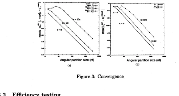
We choose thewavenumbers$k=\pi$,$2\pi$and $10\pi$and theincidentwave

as aplane wave in the $x$-axis direction $\phi=0$. For the finite element mesh, we chooseorthogonal

partition with size $(n_{r’\theta}n)$ ranging between $(2,16)$-$(2049,32768)$

.

For the standard finite element

approach, the infinite series in eigenvalues are computed until machine precision is achieved. The

resulting separable linear system is solved by using fast direct method with FFT.

The maximum errors $||u-u_{h}^{\mathrm{s}\mathrm{t}\mathrm{d}}||_{\infty,\Omega_{R}}$ ,$||u-u_{h}^{\mathrm{m}\mathrm{i}\mathrm{x}\mathrm{e}\mathrm{d}}||_{\infty,\Omega_{R}}$ against the angular partition size are

shown inFig. $3(\mathrm{a})$. The maximumerrorbetweenthe two computed solutions $||u_{h}^{\mathrm{s}\mathrm{t}\mathrm{d}}-u_{h}^{\mathrm{m}\mathrm{i}\mathrm{x}\mathrm{e}\mathrm{d}}||_{\infty,\Omega_{R}}$ is

shown in Fig. $3(\mathrm{b})$ in logarithmic scale. Both solutions convergelinearlyas wellas theirdifference.

Figure3: Convergence

6.2 Efficiency

testing

To test the computing timedifference between themethods, weconsider the first test example above

and an example with anelliptic shape obstacle with

axes

$2a=2.0$ and $2b=1.2$

.

The wavenumbe

(10)

k $=\pi$. We choose the artificial boundary radius R $=1.1$ and 3.0. The radial and angular partition

sizes $n_{r}=40$and $n_{\theta}=256$ respectively. Theresults areshown in Table 1.

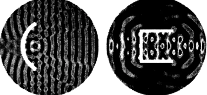
We also considered

an arc

shapedobstacleand the Helmholtz resonator with the domaintruncated

ed by inner and outerartificial boundaries. The scattering

waves

and thefar-fieldpattern

are

com-puted by using theformulafor solutionoutsidethe computational domain. Fromthefar-fieldpattern,

the radar crosssection (RCS) is computedbyusing theformula$RCS(\theta)=10\log_{10}(\omega|F(\theta)|^{2})$ which

is in decibel units [7]. The total

waves

(real part) for circulararc with waves number $k=6\pi$ _and

scattering waves (real part) for the Helmholtz resonator withwave number $k=3\pi$ _{and their radar}

cross sections are shown inFig. 4.

Figure4: Wavepatternfor antenna and Helmholtz resonator

Figure 5: Radar

cross

sectionsfor antennaand Helmholtz resonator

7 Conclusions

In this paper, we proposed amixed type method for the finite element approximation of non-local

radiation boundary condition written in the form of pseudo differential operator. We defined a

mixed tyPe approximationmatrix to approximatethesesqui-linear form corresponding to the$\mathrm{D}\mathrm{t}\mathrm{N}$

operator. The method is also efficiently applied to compute the solution ofthe radiation problem

outside the computational domain and tocompute thefar-fieldpattern.

Numerical testsshow that the mixedtyPemethod is computationally efficient. Theconvergence

is confirmed for the mixed tyPe method and is observed to be of the

same

order

as

the standard

finite element approximation

(11)

References

[1] Borgers, C, Atriangulation algorithm for fast elliptic solvers based on domain imbedding,

SIAM J. Numer. Anal. 27 No. 5, (1990) 1187-1196.

[2] Braess, D., Finite Elements, Theory, Fast Solvers and Applications in Solid Mechanics,

(Cam-bridge University Press, 1997).

[3] Ciarlet,P. G. andLions,J. L.,Handbook

_of

NumericalAnalysis, VolII, Finiteelementmethods,

(NorthHolland, 1991).

[4] Ernst,

0.

G., Afinite-element capacitance matrix method for exterior Helmholtz problems,

Numer. Math. 75, No. 2, (1996) 175-204.

[5] Freund, R. W., ATranspose-Free quasi-minimal residual algorithm for non-Hermitian linear

systems, SIAMJ. Sci. Comput. 14, (1993) 470-482.

[6] Givoli, D., Non-reflecting boundaryconditions, J. Comput. Phys. 94, (1991) 1-29.

[7] Heikkola, E., Kusnetsov, Y. A., Neittaanmaki, P. and ToivanenJ., Fictitiousdomain methods

for the numerical solutionof tw0-dimensionalscattering problems, J. Comput. Phys. 145, (1998)

89-109.

[8] Ihlenburg, F., Finite Element Analysis

of

AcousticScattering, Applied Mathematical Sciences,

132 (Springer-Verlag, 1998).

[9] Kako, T., Approximation of scattering state by means of the radiation boundary condition,

Math. Meth. in the Appl. Sci. 3, (1981) 506-515.

[10] Keller,J. and Givoli, D., Exact non-reflecting boundaryconditions, J. Comput. Phys. 94, (1989)

172-192.

[11] Koyama, D., Mathematical analysis of the DtN finite element method for the exterior Helmholtz

problem, Report CS 00-06, Univ. of ElectrO-Communications, 2000.

[12] Kuznetsov, Yu.A. and Lipnikov, K. N. 3DHelmoltzwaveequation by fictitious domain method,

Russ. J. Numer. Anal. Math. Modeling,13 No. 5, (1998) 371-387.

[13] Liu, X., Study

on

Approximation method for the Helmholtz equation in unbounded region,

PhD. thesis, The University of ElectrO-Communications, JaPan, 1999.

[14] Liu, X. and Kako, T., Higher order radiation boundary condition and finite element method

for scattering problem, Advances in Mathematical Sciences and Applications 8, No. 2, (1998)

801-819.

[15] Lynch, R. E., Rice, J. R. and Thomas, D., Direct solutions ofpartial differential equations by

tensor product methods, Numer. Math. 6(1964) 185-199.

[16] MacCamy,R. C, Marin, S. P. A, Finite element method for exterior interface problems.

Inter-nat. J. Math. Math. Sci. 3, No. 2, (1980) 311-350.

[17] Masmoudi, M., Numerical solution for exteriorproblems, Numer. Math. 51, (1987) 87-101.

[18] Nirenberg, L., Lecturesonlinearpartial differential equations, C. B. M. S. Regional

_Conf.

Ser.

in Math., No. 17, (Amer. math. Soc, Providence, R.I., 1973).

[19] Taylor, M. E., Pseudo

_differential

Operators, (Princeton University Press, 1981).

[20] Thompson, I. J. and Barnett, A. R., Coulomb and Besselfunctions ofcomplexargumentsand

order, J. Comput. Phys. 64, (1986) 490-509