The Reduction of a Quantum System of Three Identical Particles on a Plane (Dynamical Systems and Differential Geometry)

The

Reduction of

a

Quantum

System of

Three

Identical Particles

on

a

Plane

Toshihiro Iwai and Toru Hirose

Department of Applied Mathematics and Physics

Kyoto University

1

Introduction

In this report, a quantum $\mathrm{c}\mathrm{e}\mathrm{n}\mathrm{t}\mathrm{e}\mathrm{r}-\mathrm{o}\mathrm{f}$-mass system of three identical particles

on

a

plane is considered, and reduced to

a

system which has less degrees of

freedom. The reduction will be performed through two symmetry structures

in the system, which are;

1. rotation of all particles about the origin makes

no

difference in the

physical state of the system,

2. the system is indistinguishable when particles

are

exchanged, because

all particles are identical.

Figure 1 shows the overall idea of reduction. As

a

practical application of the

Figure 1: The configurationspaceadmits the action ofthe rotationgroupand

of the symmetric group, which are to the left and to the right respectively.

theory, a free three-particle quantum planar system is considered. On the

basis of the rotational symmetry, the $\mathrm{c}\mathrm{e}\mathrm{n}\mathrm{t}\mathrm{e}\mathrm{r}-\mathrm{o}\mathrm{f}$-mass system for the planar

three-body system is made into a principal fiber bundle $\dot{\mathrm{R}}^{4}arrow\dot{\mathrm{R}}$3 with

structure group $\mathrm{S}\mathrm{O}(2)$, where the action of the group is to the left, and the

数理解析研究所講究録

Figure 2: Three particles

are

to

move

around

on

the plane. All particles

are

labeled,

so

that exchanges ofparticles are trackable.

dot symbol indicates that the origin is removed from the space in question.

A similar process should be taken for the particle exchange symmetry, which

may be carried out in terms of the symmetric group $S_{3}$. A point to make

here is that the theory should apply to a system containing any number

of particles, and of

course can

do in three dimensions, too. The

reason

why this particular example _{is chosen is because for} systems with four or

more

particles, the symmetric group $S_{n}$ arriving from particle exchanges

gets rapidly

more

difficult to treat in an explicit manner, and we feel that

$n=3$ _{for the number ofparticles is comfortable to present the idea.}

2

Configuration Space

and Jacobi

Vectors

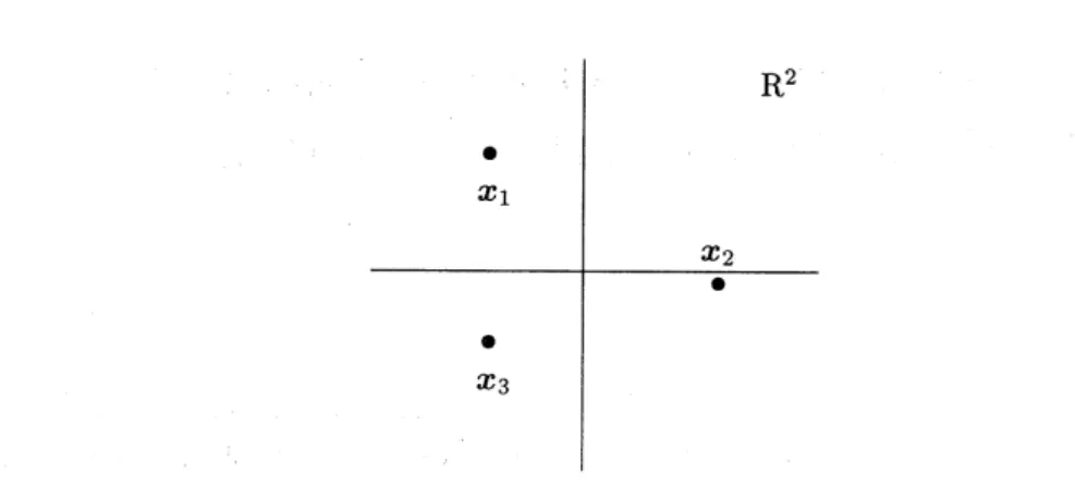
Suppose thereare threeparticles

on

aplane, each with position vectors $x_{1},$$x_{2}$,

and $x_{3}$, and

masses

$m_{1},$ $m_{2}$, and $m_{3}$, respectively. The particles are

con-strained to move on the plane, so $x_{j}\in \mathrm{R}^{2}$. The set of all possible particle

positions is identified with $X\cong \mathrm{R}^{2\cross 3}$, which consists of ordered triples of

position vectors $(x_{1}, x_{2}, x_{3})$. The position vector ofparticle 1 is entered into

the left most slot in the brackets. Figure 2 illustrates the spreaded particles

on the plane. Each particle is labeled for the time being.

Since equations of motion

are

not yet given, the particles have no

pre-scribed motions. The purpose of the current discussion is to give a rough

idea of the space that particles can lie in.

funda-mental motions traced by the particles, one of which is the translation;

$(x_{1}, x_{2}, x_{3})\mapsto(x_{1}+a, x_{2}+a, x_{3}+a)$, $a\in \mathrm{R}^{2}$, (1)

and the other is the rotation

$(x_{1}, x_{2}, x_{3})rightarrow(gx_{1}, gx_{2}, gx_{3})$, _{$g\in SO(2)$}. (2)

The space $X$ is endowed with the inner product $K$ : $X\cross Xarrow \mathrm{R}$,

$K(x, y)= \sum_{j=1}^{3}m_{j}(x_{j,y_{j}})$, $x,$$y\in X$, (3)

where $(x, y)$ denotes the standard inner producton$\mathrm{R}^{2}$

. Note that this metric

incorporates mass, which will cause later the absence of$m$, a massfactor, in

the Schr\"odinger equation. This is because the coordinate system that is to

be produced on the basis of this metric contains mass already.

We shall now focus on the $\mathrm{c}\mathrm{e}\mathrm{n}\mathrm{t}\mathrm{e}\mathrm{r}-\mathrm{o}\mathrm{f}$-mass system, which means that the

center of

mass

of the particles remains fixed at the origin;

$\sum_{1}^{3}m_{j}x_{j}=0$, (4)

and this will imply that noaction of translations is possible. We shall denote

this $\mathrm{c}\mathrm{e}\mathrm{n}\mathrm{t}\mathrm{e}\mathrm{r}-\mathrm{o}\mathrm{f}$-mass system by

$X_{0}= \{(x_{1}, x_{2}, x_{3})\in X|\sum_{j=1}^{3}m_{j}x_{j}=0\}$ (5)

The space $X$ has its natural orthonormal basis $(e_{1},0,0),$ $(e_{2},0,0),$ $\ldots$,

con-forming to the inner product defined by (3), but this does not mean that the

subspace $X_{0}\subset X$ has the

same

basis. Here $e_{j}$

are

the standard basis

vec-tors for $\mathrm{R}^{2}$

. Any basis for $X_{0}$ must satisfy the condition (4) and so must be

manually constructed by the Gram-Schmidt process. We note that the pair

$(-m_{2}e_{1}, m_{1}e_{1},0)$ and $(-m_{2}e_{2}, m_{1}e_{2},0)$ satisfies (4), and that these vectors

are

orthogonal with respect to the metric (3). Normalizing theses vectors

and using them

as

the seeds for the process, we find that

a

suitable set of

orthonormal basis vectors shall be given by

$f_{1}$ $=$ $N_{1}(-m_{2}e_{1}, m_{1}e_{1},0)$, (6)

$f_{2}$ $=$ $N_{1}(-m_{2}e_{2}, m_{1}e_{2},0)$, (7)

$f_{3}$ $=$ _{$N_{2}(-m_{3}e_{1}, -m_{3}e_{1}, (m_{1}+m_{2})e_{1})$}, (8)

$f_{4}$ $=$ $N_{2}(-m_{3}e_{1}, -m_{3}e_{2}, (m_{1}+m_{2})e_{2})$, (9)

where $N_{j}$

are

the normalizing factors explicitly given by

$N_{1}$ $=$ $(m_{1}m_{2}(m_{1}+m_{2}))^{-1/2}$, ₍₁₀₎

$N_{2}$ $=$ $(m_{3}(m_{1}+m_{2})(m_{1}+m_{2}+m_{3}))^{-1/2}$_{. (11)}

Since $f_{j},$$j=1,$

$\ldots,$$4$

are

basis vectors on $X_{0}$, any $x\in X_{0}$ can be represented

as a

linear combination of$f_{j}’ \mathrm{s}$;

$x= \sum_{j=1}^{4}q_{j}f_{j}$, $q_{j}=K(x, f_{j}))$ (12)

where $q_{j}$

are

the coefficients, and define the new coordinate system for $X_{0}$,

and in what follows we shall call the space $X_{0}$ the configuration space. The

coordinate system $(q_{j})$ will reappear later, but for the time being an

alter-native system is considered, as the new system is

more

suitable for dealing

with particle exchanges.

The space $X_{0}$ is isomorphic to $\mathrm{R}^{4}$

and also to $\mathrm{R}^{2}\cross \mathrm{R}^{2}$

, the set of pairs of

vectors in $\mathrm{R}^{2}$. We define

the pair of two vectors as follows;

$r_{1}$ $=$ (13)

$r_{2}$ $=$ $q_{3}e_{1}+q_{4}e_{2}= \sqrt\frac{m_{3}(m_{1}+m_{2})}{m_{1}+m_{2}+m_{3}}(x_{3}-\frac{m_{1}x_{1}+m_{2}x_{2}}{m_{1}+m_{2}})$ _. (14)

The vectors $r_{1}$ and $r_{2}$

are

called the Jacobi vectors. One vector is pointing

along the line between particles _{1 and 2, while the other is pointing along the}

line between particle 3 and the center ofmass ofparticles 1 and 2. Figure 3

Figure 3: Illustrating the Jacobi vectors $r_{1}$ and $r_{2}$

as seen

in Eqs. (13-14). $r_{1}$ points along the line joining particles 1 and 2, while _{$r_{2}$} points along the

line joining particles 3 and the center ofmass ofparticles 1 and 2. Note that

the

arrow

lengths

are

not drawn to scale.

3

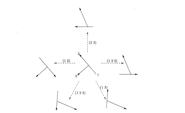
Exchanges

of Particles

It it

now

important to recall that

one

of the symmetries that is utilized to

perform the reduction is theindistinguishibilityofconfigurations arisingfrom

exchanges of identical particles. Thus in this section,

we

make all particles

identical and without loss of generality put $m_{j}=1,$$j=1,2,3$. Then the

Jacobi vectors defined in Eqs. (13-14) become

$r_{1}$ $=$ $\frac{1}{\sqrt{2}}(x_{2}-x_{1})$, (15)

$r_{2}$ $=$ $\sqrt{\frac{2}{3}}(x_{3}-\frac{x_{1}+x_{2}}{2})$ . (16)

If, for example, particles 1 and 2

are

exchanged, then the configuration

un-dergoes

a

change

$(x_{1}, x_{2}, x_{3})rightarrow(x_{2}, x_{1}, x_{3})$ . (17)

This

can

be

more

generalized.

Since

any combination ofexchanges of

parti-cles

can

beexpressed as aparmutation map$\sigma\in S_{3}$, where$S_{3}$ is thesymmetric

group oforder six, the change the configuration takes is expressed

as

$(x_{1}, x_{2}, x_{3})-(x_{\sigma(1)}, x_{\sigma(2)}, x_{\sigma(3)})$. (18)

The Jacobi vectors associated with $(x_{\sigma(1)}, x_{\sigma(2)}, x_{\sigma(3)})$ are then expressed as

$r_{1}’$ $=$ $\frac{1}{\sqrt{2}}(x_{\sigma(2)}-x_{\sigma(1)})$, (19)

$r_{2}’$ $=$ $\sqrt{\frac{2}{3}}(x_{\sigma(3)}-\frac{x_{\sigma(1)}+x_{\sigma(2)}}{2})$

.

(20)

If particles are exchanged in the manner of (17), then visually the direction

of the

arrow

drawn to represent $r_{1}$ is reversed. Bearing this in mind, one

soon

realizes that any combination of particle exhcnages can be represented

by a linear transformation of Jacobi vectors $r_{1}$ and $r_{2}$. This will imply that

this center-of-mass system of three identical particles admits the action of$S_{3}$

to the right. As in the

case

of example (17),

one

finds that the

new

pair of

Jacobi vectors after the particle exhcnage is given by

$(r_{1}’, r_{2}’)=(r_{1}, r_{2})$

.

(21)

Ifone works through all possible combinations of exchanges, one will find the

correspondence of permutations with linear transformation matrices. The

graphical representation of this is simply given in Figure 4 indicating which

transformation takes the reference Jacobi vectors to which pair ofnew Jacobi

vectors. We have to note here that we are dealing with the right action of

matrices, which is expressed as

$(r_{1}, r_{2})A=( \sum_{j=1}^{2}r_{j}a_{j1}, \sum_{j=1}^{2}r_{j}a_{j2})$ for $A=(a_{ji})$, (22)

and has the property

$((r_{1}, r_{2})A)B=(r_{1}, r_{2})(BA)$. (23)

Hence, the representation of$S_{3},$ $\rho$

:

$S_{3}arrow GL(2, \mathrm{R})$ that is required to satisfy

$\rho(g_{1}g_{2})=\rho(g_{1})\rho(g_{2})$ for $g_{1},$$g_{2}\in S_{3}$, must act on $X_{0}$ in the manner

Figure 4: This diagram represents the graphical view of all possible particle

exchanges. Numbers in brackets are the elements of permutations from $S_{3}$.

A straightforward calculation then provides

$\rho(e)$ $=$

$\rho(123)$ $=$ $(-\sqrt{3}/2-1/2$ $\sqrt{3}/2-1/2)$ , $\rho(132)$ $=$ $(\sqrt{3}/2-1/2$ $-\sqrt{3}/2-1/2)$ ,

$\rho(23)$ $=$ $(\sqrt{3}/21/2$ $\sqrt{3}/2-1/2)$ , $\rho(13)$ $=$ $(-\sqrt{3}/21/2$ $-\sqrt{3}/2-1/2)$ _.

(25)

It is

an

easy matter to verify that the matrices in (25) form a discrete

sub-group of $0(2)$ which is isomorphic to the symmetric

group

$S_{3}$.

Implementing this for

an

$n$-particle system with $n\geq 4$ is not

an

easy

task, as we have alluded in Introduction.

4

The Internal Space

What was established in Sec.3, was to describe the action of$S_{3}$ onthe

center-of-mass system, which comes from exchanges of particles. In this section,

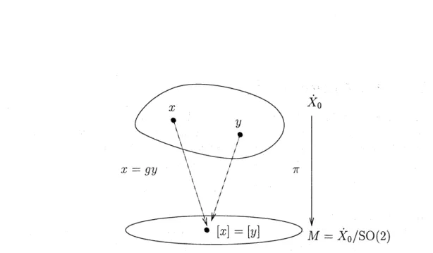
the symmetry due to the rotation is considered. Having removed the

trans-lational degrees of freedom,

we can now

consider the relative positions of the

particles. If a given configuration of particles $x\in X_{0}$ is rotated about the

origin and is found to fit another configuration $y\in X_{0}$, say, then $x$ and $y$ are

said to be ((

$\mathrm{s}\mathrm{i}\mathrm{m}\mathrm{i}\mathrm{l}\mathrm{a}\mathrm{r}$” and there exists a linear

transformation $g\in \mathrm{S}\mathrm{O}(2)$ such

that $x=gy$. For convenience, we forget the case where all _{particles collide}

at the origin, and consider the configuration space $\dot{X}_{0}:=X_{0}-\{0\}$ in the

following. Here the $\mathrm{e}\mathrm{x}\mathrm{p}\mathrm{l}\mathrm{i}\mathrm{c}\mathrm{i}\mathrm{t}$expression of the

$g$ action is given by;

$x=(x_{1}, x_{2}, x_{3})\mapsto(gx_{1}, gx_{2}, gx_{3})=gx$, $g\in \mathrm{S}\mathrm{O}(2),$ $x\in\dot{X}_{0}$, (26)

and the ((

$\mathrm{s}\mathrm{i}\mathrm{m}\mathrm{i}\mathrm{l}\mathrm{a}\mathrm{r}\mathrm{i}\mathrm{t}\mathrm{y}$

” _of

$x$ and $y$ can be easily shown to be an equivalence

relation;

$x\sim y$ if and only if $x=gy$ . (27)

Then there exists the natural projection $\pi$ from the configuration space to

the quotient space,

$\pi$ : $\dot{X}_{0}arrow M:=\dot{X}_{0}/\mathrm{S}\mathrm{O}(2)$, (28)

which is defined to be

$\pi(x)=[x]$, $x\in X_{0}$, (29)

where $[x]$ denotes the equivalence class of $x$. The space $M$ in (28)

con-tains all possible inequivalentclasses with respect to the equivalence relation

(27). Physically, the elements of$M$ express labels of different triangle shapes

formedby $(x_{1}, x_{2}, x_{3})$ without counting the duplicated ones due to rotations

about the origin.

In addition, $M$ turns out to be

a

manifoldwhich we shall call the internal

or

shape space, and $\dot{X}_{0}$ is made into

a

fiber bundle. A

graphical view of this

projection (28) is presented in figure 5.

To elaborate the discussion,

we

wish to give the explicit form of the

Figure 5: The projection $\pi$ takes two equivalent configurations to the

same

equivalent class in $M$. In reality, $x$ and $y$ are on the same fiber.

space $\dot{X}_{0}$,just as

was

previously defined. We notice that _{$X_{0}$} can be identified

with $\mathrm{C}^{2}$ by introducing the complex vriables

$z_{1},$ $z_{2}$ through

$z_{1}$ $=$ $q_{1}+iq_{2}$, (30)

$z_{2}$ $=$ $q_{3}+iq_{4}$. (31)

We work in terms of the new coordinates. On account of (13), (14), and

(26) with

$g=$

, the action of SO(2) on $\mathrm{C}^{2}$ turns out to be

expressed

as

$z=(z_{1}, z_{2})\mapsto(e^{it}z_{1}, e^{it}z_{2})=e^{it}z$. (32)

Here$t$is not considered

as

the temporal variable, but as

a

parameter ofSO(2).

With the identification $X_{0}\cong \mathrm{C}^{2}$, the natural projection $\pi$ is expressed as

$\pi$ : $(z_{1}, z_{2})rightarrow(\xi_{1}, \xi_{2}, \xi_{3})$, (33)

where

$\xi_{1}+i\xi_{2}$ $=$ $2z_{1}\overline{z}_{2}$, (34) $\xi_{3}$ $=$ $|z_{1}|^{2}-|z_{2}|^{2}$. (35)

It

can

be verified that the internal space $M$ is diffeomorphic with $\dot{\mathrm{R}}^{3}\mathrm{w}$

, hich

is $\mathrm{R}^{3}$ with the origin removed,

$M:=\dot{X}_{0}/\mathrm{S}\mathrm{O}(2)\cong\dot{\mathrm{R}}^{3}:=\mathrm{R}^{3}-\{0\}$ . (36)

5

The Action of

$S_{3}$

on

$M$

In Section 3, we have observed that the exchanges of identical particles give

rise to the action of $S_{3}$ on $X_{0}$, and $S_{3}$ turned out to be represented as a

discrete subgroup of $\mathrm{O}(2)$ consisting of six elements. With the identification

$X_{0}\cong \mathrm{C}^{2}$, the action of $S_{3}$

on

$X_{0}$ is expressed

as

$(z_{1}, z_{2})-+(z_{1}, z_{2})\rho(h)^{-1}$, $h\in S_{3}$, (37)

as

is seen from (24).

We now consider how this action behaves

on

the internal space $M$. For

$h\in S_{3}$, the associated matrix $\tau(h)$ is defined by

$[x\rho(h)^{-1}]:=[x]\tau(h)^{-1}$, $[x]\in M$. (38)

Note here that this definition is independent of the choice ofrepresentatives.

From (34-35) together with (37-38), the symmetric group $S_{3}$ is shown to act

on $M$ to the right;

$(\xi_{1}, \xi_{2}, \xi_{3})-+(\xi_{1}, \xi_{2}, \xi_{3})\tau(g)^{-1}$, $g\in S_{3)}$ (39)

where $\tau$ is

a

representation $\tau$ : $S_{3}arrow \mathrm{G}\mathrm{L}(3, \mathrm{R})$. A straightforward calculation

shows that $\tau(S_{3})$ forms

a

discrete subgroup of $\mathrm{S}\mathrm{O}(3)$, which is expressed

as

$\tau(e)$ $=$

$\tau(123)$ $=$ $(\sqrt{3}/2-1/20$ $001$ $-\sqrt{3}/2-1/20)$ , $\tau(132)$ $=$ $(-\sqrt{3}/2-1/20$ $001$ $\sqrt{3}/2-1/20)$ ,

$\tau(23)$ $=$ $(\sqrt{3}/21/20$ $-100$ $\sqrt{3}/2-1/20)$ , $\tau(13)$ $=$ $(-\sqrt{3}/21/20$ $-100$ $-\sqrt{3}/2-1/20)$

(40)

It is of interest to observe that the matrices acting on $M$ have the unit

determinant while those acting

on

$X_{0}$ have determinants either 1

or

$-1$. At

first sight, the dimension of matrices presented in (40) is 3 $\cross 3$, which is

larger than those presented in (25), resulting an increase in the number of

is less than that of$\dot{X}_{0}$. However, this is not

a

contradiction. While we have

identified $X_{0}$ with $\mathrm{R}^{2\cross 2}$, the set of Jacobi vectors, we

are

allowed to identify

$X_{0}$ with $\mathrm{R}^{4}$

, the set ofrow vectors of length 4, so that we would have seen a

discrete subgroup of$\mathrm{G}\mathrm{L}(4, \mathrm{R})$ acting, and have been able tosee an immediate

reduction in the size of matrices. In fact, the $\mathrm{O}(2)$ action given in (24) proves

to take the form

$(q_{1}, q_{2}, q_{3}, q_{4})-arrow(q_{1}, q_{2}, q_{3}, q_{4})$ for

$\rho(g)=$

, (41)

where $g\in S_{3}$ and $I_{2}$ denotes the $2\cross 2$ unit matrix. Thus we also

see

that the

determinant ofthe $4\cross 4$ matrix in the above is the square ofthe determinat

of the 2 $\mathrm{x}2$ matrix _$\rho(g)$, that is, unity,

so

that the $S_{3}$ is represented

as a

discrete subgroup of$\mathrm{S}\mathrm{O}(4)$.

6

Reduction

by

Rotation Symmetry

In this section, we present the reduction of the system of three free particles

by rotation symmetry. The reduction goes through irrespective of whether

all three particles are identical or not. The Schr\"odinger equation for free

particles we consider here is given by

$i \hslash\frac{\partial\psi}{\partial t}=-\frac{\hslash^{2}}{2}\nabla^{2}\psi$

with $\nabla^{2}=\sum_{j=1}^{4}\frac{\partial^{2}}{\partial q_{j}^{2}}$. (42)

In fact, since the oprator $\sum_{k=1}^{3}(1/m_{k})(\partial/\partial x_{k})^{2}$ is the Laplacian with respect

to the metric (3) on $X$, and since this metric is expressed

as

$\sum_{j=1}^{4}dq_{j}^{2}$ if

restricted to the linear subspace $X_{0}$ of $X$,

so

that

our

Laplacian takes the

form of $\nabla^{2}=\sum_{j=1}^{4}\partial^{2}/\partial q_{i}^{2}$ in the coordinates $(q_{j})$. As is well known, this

equation

can

be solved by Fourier transform with little difficulty, to give

solution of the form

$\psi(z, t)=\int_{\mathrm{C}^{2}}G(z, t,\cdot w, t_{0})\psi_{0}(w, t_{0})dw$, (43)

where $G$ is the Green function, of which the explicit form is given by

$G(z, t;w, t_{0})=[ \frac{1}{2\pi ih(t-t_{0})}]^{2}\exp(\frac{i|z-w|^{2}}{2h(t-t_{0})})$. (44)

By $|z-w|^{2}$, we mean the Euclidian distance in $\mathrm{C}^{2}$ ; $|z-w|^{2}$ $=$ $|z_{1}-w_{1}|^{2}+|z_{2}-w_{2}|^{2}$ (45) $=$ $\sum_{j=1}^{4}(q_{j}-p_{j})^{2}$, (46) where $w_{1}$ $=$ $p_{1}+ip_{2}$, (47) $w_{2}$ $=$ $p_{3}+ip_{4}$, (48)

and $q_{j}’ \mathrm{s}$ as previously defined in (30-31).

Since the Schr\"odinger equation (42) is invariant under the $\mathrm{S}\mathrm{O}(2)$ action

(32), the free particle system will be shown to be reduced to a system on

$\mathrm{t}_{J}\mathrm{h}\mathrm{e}$ internal space $M$

. Before proceeding with the reduction, we need a

decomposition of $L^{2}(\mathrm{C}^{2})$ with the $\mathrm{S}\mathrm{O}(2)$ action. For $f\in L^{2}(\mathrm{C}^{2})$ given,

we

consider a function $f(e^{is}z)$ with a parameter $s$, which can be expanded into

the Fourier series

$f(e^{is}z)= \sum_{m=-\infty}^{\infty}f_{m}(z)e^{ims}$, $f_{m}(z)= \frac{1}{2\pi}\int_{-\pi}^{\pi}f(e^{is}z)e^{-ims}ds$. (49)

In particular, we have, for $s=0$,

$f(z)= \sum_{m=-\infty}^{\infty}f_{m}(z)$. (50)

Note that the function $f_{m}$ defined in (49) satisfies $f_{m}(e^{is}z)=e^{ims}f_{m}(z)$_. Any

function $f$ on $\mathrm{C}^{2}$ satisfying the equation

$f(e^{\iota s}z)=e^{\iota ms}f(z)$ (51)

is called $\rho_{m}$-equivariant, where $\rho_{m}$ denotes a unitary irreducible

representa-tion of SO(2) $\cong \mathrm{U}(1),$ $\rho_{m}(e^{is})=e^{ims}$. On account of the invariance of the

Lebesgue measure $dz$ on $\mathrm{C}^{2}$ under the

$\mathrm{S}\mathrm{O}(2)$ action, we can verify in the $L^{2}$

norm that

which implies that $L^{2}(\mathrm{C}^{2})$ can be decomposed into the direct sum of $L_{m}^{2}$’s;

$L^{2}( \mathrm{C}^{2})=\bigoplus_{m=-\infty}^{\infty}L_{m}^{2}(\mathrm{C}^{2})$ , (53)

where

$L_{m}^{2}(\mathrm{C}^{2})=\{f\in L^{2}(\mathrm{C}^{2})|f(e^{is}z)=e^{ims}f(z)\}$. (54)

We note that $f_{m}\in L_{m}^{2}(\mathrm{C}^{2})$.

Our task in the following is to decompose the time evolution (43) in

$L^{2}(\mathrm{C}^{2})$ intoaseriesof those in respective subspaces $L_{m}^{2}(\mathrm{C}^{2})$. This process will

be called the reduction of the free particle system for simplicity. We will

see

later how the time evolution in $L_{m}^{2}(\mathrm{C}^{2})$ is looked upon as the time evolution

ofastate on the internal space$M$. However, before performing the reduction,

it is rather necessary to

see a

few properties of this Green’s function and the

integral transform. For the purpose of easier reading,

we

shall write simply

$G_{t}(z, w)$ and $\psi_{t}(z)$ for $G(z, t;w, t_{0})$ and $\psi(z, t)$, respectively. Then $G_{t}(z, w)$

is invariant under the SO(2) action to the left defined in (32);

$G_{t}(e^{is}z, e^{is}w)=G_{t}(z, w)$, (55)

which is equivalent to the invariance of the Laplacian $\nabla^{2}$. Further, the

integral transform with the Green’s kernel$G_{t}(z, w)$ has thefollowingproperty

for any $s\in \mathrm{R}$

$\int_{\mathrm{C}^{2}}G(z, w)\psi_{0}(w)dw=\int_{\mathrm{C}^{2}}G(z, e^{-is}w)\psi_{0}(e^{-is}w)dw$, (56)

since the Lebesgue

measure

$dw$ is invaraint under the $\mathrm{U}(1)$ action, $w\vdasharrow e^{is}w$.

For $\psi_{0}\in L^{2}(\mathrm{C}^{2})$ given, $\psi_{0}(e^{is}w)$ can be expanded into Fourier series, $\psi_{0}(e^{is}w)=\sum_{m=-\infty}^{\infty}\psi_{0}^{m}(w)e^{ims}$ where $\psi_{0}^{m}(w)=\frac{1}{2\pi}\int_{-\pi}^{\pi}\psi_{0}(e^{is}w)e^{-ims}ds$.

(57)

Using the above properties and the expansion, we obtain

$\psi_{t}(z)$ $=$ $\int_{\mathrm{C}^{2}}G_{t}(z, w)\psi_{0}(w)dw$ (58)

$=$ $\frac{1}{2\pi}\int_{-\pi}^{\pi}ds\int_{\mathrm{C}^{2}}G_{t}(z, w)\psi_{0}(w)dw$ (59) $=$ $\frac{1}{2\pi}\int_{-\pi}^{\pi}ds\int_{\mathrm{C}^{2}}G_{t}(z, e^{-is}w)\psi_{0}(e^{-is}w)dw$ (60) $=$ $\frac{1}{2\pi}\int_{-\pi}^{\pi}ds\int_{\mathrm{C}^{2}}G_{t}(z, e^{-is}w)\sum_{m=-\infty}^{\infty}\psi_{0}^{m}(w)e^{-ims}dw$ (61) $=$ $\sum_{m=-\infty}^{\infty}\int_{\mathrm{C}^{2}}G_{t}^{m}(z, w)\psi_{0}^{m}(w)dw$, (62) where $G_{t}^{m}(z, w):= \frac{1}{2\pi}\int_{-\pi}^{\pi}G(e^{is}z, w)e^{-ims}ds$, (63)

and assuming that the order of integration and summation

can

be

inter-changed safely, which is the

case

for $f\in S(\mathrm{C}^{2})$, rapidly decreasing $C^{\infty}$

func-tions. The $G_{t}^{m}(z, w)$ in (63) is the Green’s kernel which operates

on

$L_{m}^{2}(\mathrm{C}^{2})$.

.

At

a

glance of $G_{t}^{m}(z, w)$,

we

may expect it to have properties that

are

likes

of equivariance. In fact, we can show that

$G_{t}^{m}(e^{is}z, w)$ $=$ $e^{ims}G_{t}^{m}(z, w)$, (64) $G_{t}^{m}(z, e^{is}w)$ $=$ $e^{-ims}G_{t}^{m}(z, w)$, (65)

which

means

that $G_{t}^{m}(z, w)$ is equivariant with respect to the $\mathrm{U}(1)$ action

on

$z$, and is anti-equivariant with respect to that on $w$. Thus we have

de-composed the time evolution of the original system in $L^{2}(\mathrm{C}^{2})$ into a series of

those in $L_{m}^{2}(\mathrm{C}^{2})$, accomplishing the reduction, as is expressed in (62).

Carrying

on

from the last passage, (63) can be explicitely computed to

give

where $J_{m}$ is the Bessel function and

$B(z, w)$ $=$ $\sum_{j=1}^{2}(|z_{j}|^{2}+|w_{j}|^{2})$ for $z_{j},$$w_{j}\in \mathrm{C}$, (67)

$A(z, w)$ $=$ $2|z_{1}\overline{w}_{1}+z_{2}\overline{w}_{2}|$, (68)

$\theta(z, w)$ $=$ $\arg\sum_{j=1}^{2}z_{j}\overline{w}_{j}$. (69)

It is ofgreat interst to observe that $A(z, w)$ and $B(z, w)$

can

be expressed in

the coordinates of the internal space $M$. In fact, we

can

verify that

$B(z, w)$ $=$ (70)

$A(z, w)$ $=$ $[ \frac{1}{2}\uparrow\sum_{k=1}^{3}\xi_{k\uparrow 2}^{2}\sum_{k=1}^{3}\xi_{k}’+\frac{1}{2}\sum_{k=1}^{3}\xi_{k}\xi_{k}’]^{1/2}$, (71)

where $\xi_{k}’$

are

given by the formulae

$\xi_{1}’+i\xi_{2}’$ $=$ $2w_{1}\overline{w}_{2}$, (72)

$\xi_{3}’$ $=$ $|w_{1}|^{2}-|w_{2}|^{2}$. (73)

We notice further that under the $\mathrm{S}\mathrm{O}(2)$ action $z\vdasharrow e^{is}z$ (resp., $w-te^{is}w$),

the factor $e^{im\theta(z,w)}$ is subject to the transformation $e^{im\theta(z,w)}\mathrm{f}\Rightarrow e^{ims}e^{im\theta(z,w)}$

(resp., $e^{im\theta(z,w)}rightarrow e^{-ims}e^{im\theta(z,w)}$).

7

Symmetry due

to

Particle Exchanges

This section deals with identical particles. According to whether particles

are all bosons or fermions, the wave function must be symmetric or

antisym-metric with respect to

a

particle interchange. For our three-particle system,

according as paprticles are all bosons or fermions, the wave function $\psi$ on

the center-of-mass sytem must satisfy

$\psi(x_{\sigma(1)}, x_{\sigma(2)}, x_{\sigma(3)})=\psi(x_{1}, x_{2}, x_{3})$ for $\sigma\in S_{3)}$

or

(74) $\psi(x_{\sigma(1)}, x_{\sigma(2)}, x_{\sigma(3)})=\mathrm{s}\mathrm{g}\mathrm{n}(\sigma)\psi(x_{1}, x_{2}, x_{3})$ for $\sigma\in S_{3}$, (75)

where sgn denotes the signum of $\sigma;\mathrm{s}\mathrm{g}\mathrm{n}(\sigma)$ equals 1 of $-1$, depending on

whether $\sigma$ is an even or odd permutation. In particular, afunction satisfying

(75) is called satisfying the Pauli principle. For a wave function $\psi$ on the

configuration space $\mathrm{C}^{2}$, one can construct a wave

function satisfying the

above respective symmetry by the following procedures,

$\psi^{(s)}(x):=\sum_{h\in S_{3}}\psi(x\rho(h)^{-1})$, (76)

$\psi^{(a)}(x):=\sum_{h\in S_{3}}\mathrm{s}\mathrm{g}\mathrm{n}(h)\psi(x\rho(h)^{-1})$, (77)

where$\rho$ is the representationof$S_{3}$ in $\mathrm{O}(2)$. The $\psi_{s}$ and$\psi_{a}$ indeed satisfy (74)

and (75), respectively. We note that $G_{t}(z, w)$ is invariant under the action

of$h\in S_{3}$ on account of the very definition (44) together with (41);

$G_{t}(z\rho(h)^{-1}, w\rho(h)^{-1})=G_{t}(z, w)$, (78)

which is equivalent to the invariance of the Laplacian $\nabla^{2}$ under the action

of$S_{3}$. This invariance together with the invariance of the Lebesgue measure

$dw$ under the action of $S_{3}$ will imply that the time evolution preserves the

statistics to which theparticles aresubject, that is, bosonic orfermionic state

remains preserved during the time evolution. In fact, for the action of $S_{3)}$

the time evolution (58) of the initial state undergoes the change

$\psi_{t}(z\rho(h)^{-1})$ $=$ $\int_{\mathrm{C}^{2}}G_{t}(z\rho(h)^{-1}, w)\psi_{0}(w)dw$ (79)

$=$ $\int_{\mathrm{C}^{2}}G_{t}(z, w\rho(h))\psi_{0}(w)dw$ (80)

$=$ $\int_{\mathrm{C}^{2}}G_{t}(z, w)\psi_{0}(w\rho(h)^{-1})dw$, (81)

which implies that according to whether$\psi_{0}(h\rho(h)^{-1})=\psi_{0}(z)$ or$\psi_{0}(z\rho(h)^{-1})=$

$\mathrm{s}\mathrm{g}\mathrm{n}(h)\psi_{0}(z)$ initially, we have for all time $t$

$\psi_{t}(z\rho(h)^{-1})=\psi_{t}(z)$ or $\psi_{t}(z\rho(h)^{-1})=\mathrm{s}\mathrm{g}\mathrm{n}(h)\psi_{t}(z)$. (82)

Since the action of SO(2) and of $S_{3}$ commute, the time evolution (81) is

decomposed into

$\psi_{t}(z\rho(h)^{-1})=\sum_{m=-\infty}^{\infty}?l_{t}^{)^{m}}(z\rho(h)^{-1})=\sum_{m=-\infty}^{\infty}\int_{\mathrm{C}^{2}}G_{t}^{m}(z, w)\psi_{0}^{m}(w\rho(h)^{-1})dw$.

Putting (83) together with (76) and (77), we obtain the time evolution of

bose or fermi particles in the form,

$\psi_{t}^{(s)}(z)=\sum_{m=-\infty}^{\infty}\sum_{h\in S_{3}}\psi_{t}^{m}(z\rho(h)^{-1})$, (84)

$\psi_{t}^{(a)}(z)=\sum_{m=-\infty}^{\infty}\sum_{h\in S_{3}}\mathrm{s}\mathrm{g}\mathrm{n}(h)\psi_{t}^{m}(z\rho(h)^{-1})$ (85)

respectively.

8

Complex

line

bundles

The time evolution $\psi_{t}$ in $L^{2}(\mathrm{C}^{2})$ was decomposed into the series ofthose in

$L_{m}^{2}(\mathrm{C}^{2})$,

$\psi_{t}^{m}(z):=\int_{\mathrm{C}^{2}}G_{t}^{m}(z, w)\psi_{0}^{m}(w)dw$, $\psi_{0}^{m}\in L_{m}^{2}(\mathrm{C}^{2})$. (86)

Since $G_{t}^{m}$ and $\psi_{0}^{m}$

are

anti-equivariant and quivariant, respectively, under the

$\mathrm{S}\mathrm{O}(2)$ action $w$ -; $e^{is}w$, the integrand in (86) is invariant under the $\mathrm{S}\mathrm{O}(2)$

action,

so

that the integration with respect to $w$ over $\mathrm{C}^{2}$ will reduce to that

over the internal space $M$_. Hence the time evolution $\psi_{t}^{m}(z)$ may define the

time evolution ofa quantum state on the internal space $M$. To discuss this

evolution strictly,

we

must introduce the notion of complex line bundles.

For a unitary irreducible representation $\rho_{m}$ of SO(2) $\cong \mathrm{U}(1),$ $\rho_{m}(e^{i.s})=$

$e^{ims}$, the complex line bundle $E_{m}$ associated with the $\mathrm{S}\mathrm{O}(2).\mathrm{b}\mathrm{u}\mathrm{n}\mathrm{d}\mathrm{l}\mathrm{e}X_{0}\cong$

$\dot{\mathrm{C}}^{2}$

a

_$M$ is defined to be the quotient of the product space $X_{0}\cross \mathrm{C}$ by the

equivalence relation defined through $(z, ()\sim(e^{is}z, e^{ims}\zeta)$ for $(z, \zeta)\in\dot{\mathrm{C}}^{2}\cross$ C.

By $[(z, \zeta)]$ andby $\pi_{m}$ wedenote theequivalenceclass in $E_{m}$ andthe projection

$E_{m}arrow M$, respectively, so that one has $\pi_{m}([(z, \zeta)])=\pi(z)$. A section $\sigma$ in

$E_{m}$ is a map $Marrow E_{m}$ such that $\pi_{m}\circ\sigma=\mathrm{i}\mathrm{d}_{hI}$, where $\mathrm{i}\mathrm{d}_{M}$ is the identity

map of $M$. Then any $\rho_{m}$-equivariant function $f$ on

$\dot{X}_{0}$ determines a section $\sigma$ in $E_{m}$ by

$\sigma(\pi(z))=[(z, f(z))]$. (87)

Sections

and equivariant functions

are

in one-to-one correspondence. For sections $\sigma_{1)}\sigma_{2}$ corresponding to respective $\rho_{m}$-equivariant functions $f_{1},$ $f_{2}$,

the inner product $\langle\sigma_{1}, \sigma_{2}\rangle$ is defined through

$\langle\sigma_{1}, \sigma_{2}\rangle=\int_{M}(\sigma_{1}, \sigma_{2})d\mu_{M}=\int_{\mathrm{C}^{2}}\overline{f_{1}(z)}f_{2}(z)dz$, (88)

where $(\sigma_{1}, \sigma_{2})$ denotes the inner product in each fiber $\pi_{m}^{-1}(\pi(z))\cong \mathrm{C}$, and

$d\mu_{M}$ is the

measure on

$M$ defined for any function $\chi$

on

$M$ through the

equation

$\int_{M}\chi(p)d\mu_{M}=\int_{\mathrm{C}^{2}}\chi(\pi(z))dz$ with $\pi(z)=p$. (89)

By the definition ofthe inner product for sections,

we

see

that any

func-tion $f\in L_{m}^{2}(\mathrm{C}^{2})$ determines a square integrable section in $E_{m}$. For the

equivariant function $\psi_{t}^{m}(z)$ given in (86),

one

has the time evolution of the

corresponding section $\sigma_{t}^{m}$ in $E_{m}$,

$\sigma_{t}^{m}(\pi(z))=[(z, \psi_{t}^{m}(z))]$. (90)

Since the time evolution $\psi_{t}$ is unitary, that is, $||\psi_{t}||=||\psi_{0}||$, in particular,

$||\psi_{t}^{m}||=||\psi_{0}^{m}||$, the time evolution of the corresponding section $\sigma_{t}^{m}$ is also

unitary, that is, $||\sigma_{t}^{m}||=||\sigma_{0}^{m}||$ for all time $t$.

The $S_{3}$ action on $L_{m}^{2}(\mathrm{C}^{2})$ can be transferred to that

on

square integrable

sections in $E_{m}$. From (84) and (85),

we

obtain corresponding time evolutions

in $E_{m}$, respectively,

$\sum_{h\in S_{3}}\sigma_{t}^{m}(\pi(z)\tau(h)^{-1})$, (91)

$\sum_{h\in S_{3}}\mathrm{s}\mathrm{g}\mathrm{n}(h)\sigma_{t}^{m}(\pi(z)\tau(h)^{-1})$. (92)

The reduction is thus completed for the time evolution of free three

iden-tical particles on

a

plane. We have to stress here that we have made full use

of the symmetry arising from both the rotation and the particle exchanges

in order to obtain the above equations. We found that the key to the

re-duction by the action of$\mathrm{S}\mathrm{O}(2)$ was the formation of$f_{m}(z)\in L_{m}^{2}(\mathrm{C}^{2})$, which

was

obtained by operating $\mathrm{U}(1)$

on

$z$ and then integrating $f(e^{is}z)e^{-ims}$ with

respect to the group variable $s$, as

was seen

in (49), and that $f_{m}$ is in-one-one

correspondence with asection in $E_{m}$ which describes a quantum state on the

of the formation of $f_{m}$. In fact, particle exchanges were performed by first

operating $h\in S_{3}$ on $z$ and then instead of integrating, discrete sum was

taken for $\psi(\sigma(z)\tau(h)^{-1})$ or for $\mathrm{s}\mathrm{g}\mathrm{n}(h)\psi(\sigma(z)\tau(h)^{-1})$. We may say that this

procedure is a form of reduction, while no degrees of freedom are lowered.

These two procedures have been put together to yield (91) and (92).

9

Remarks

Let

us

be reminded that $\psi_{t}^{m}$, which is put in the integral transform given by

(86), has determined $\sigma_{t}^{m}$, which describes the time evolution of

a

quantum

state

on

the internal space $M$,

as

is

seen

in (90). In view ofthis, we would

like to attempt to put (90) in the following integral transform,

$\sigma_{t}^{m}(\pi(z))$ $=$ $[(z, \int_{\mathrm{C}^{2}}G_{t}^{m}(z, w)\psi_{0}^{m}(w)dw)]$ (93)

$=$ $\int_{M}K_{t}^{m}(\pi(z), \pi(w))\sigma_{0}^{m}(\pi(w))d\mu_{M}$. (94)

However, the integral transform in (94) is purely symbolical. In fact, the

existence of the Green kernel $K_{t}^{m}$ and the way to define integrals for sections

are not sure yet. In spite of this, we have already observed in Sec. 8 that

the time evolution $\sigma_{t}^{m}$ is unitary, so that we see that there exists a unitary

operator $U_{t}^{m}$ such that $\sigma_{t}^{m}=U_{t}^{m}\sigma_{0}^{m}$, where $U_{t}^{m}$ acts

on

square integrable

sections in $E_{m}$.

In conclusion,

we

try to express the integral transform (86)

as an

integral

on the

_{internal.space}

$M$ explicitly. To this end, we

use

local sections in the

SO(2) bundle $X_{0}arrow M$, which are defined to be

$\sigma_{+}(\xi)=(\frac{\sqrt{r+\xi_{3}}}{\sqrt{2}},$

$\frac{\xi_{1}-i\xi_{2}}{\sqrt{2(r+\xi_{3})}})$ for $\pi(z)=\xi\in D_{+}$, (95)

$\sigma_{-}(\xi)=(\frac{\xi_{1}+i\xi_{2}}{\sqrt{2(r-\xi_{3})}},$$\frac{\sqrt{r-\xi_{3}}}{\sqrt{2}})$ for $\pi(z)=\xi\in D_{-}$, (96)

where $r^{2}=\xi_{1}^{2}+\xi_{2}^{2}+\xi_{3}^{2}$, and $D_{\pm}$ are domains in $M$ defined, respectively, to

be

$D_{+}=\{\xi\in\dot{\mathrm{R}}^{3}|\xi_{3}+r\neq 0\}$, (97)

$D_{-}=\{\xi\in\dot{\mathrm{R}}^{3}|\xi_{3}-r\neq 0\}$. (98)

In the intersection $D_{+}\cap D_{-}$, one has the transformation

$\sigma_{-}(\xi)=\frac{\xi_{1}+i\xi_{2}}{\sqrt{\xi_{1}+\xi_{2}^{2}}}\sigma_{+}(\xi)$ , $\xi\in D_{+}\cap D_{-}$. (99)

By using the section $\sigma_{+}$, points of $\pi^{-1}(D_{+})$ are expressed as $z=e^{i\phi}\sigma_{+}(\xi)$

with $\xi=\pi(z),$ $\phi$beingan angle variable. Then, for a

$\rho_{m}$-equivariant function

$f$on $\pi^{-1}(D_{+})$, we obtain$f(z)=e^{im\phi}f(\sigma_{+}(\xi))$, anexpression in terms of local

coordinates $(\xi_{j}, \phi)$ in $\pi^{-1}(D_{+})$.

We first devide $M$ into a disjoint union $M=M_{+}\cup M_{-}$, where $M_{\pm}$

are

the upper and the lower half space of $M\cong\dot{\mathrm{R}}^{3}$

. Accordingly, the integral

transform (86) is broken up into

$\psi_{t}^{m}(z)$ $=$ $\int_{\pi^{-1}(M)}G_{t}^{m}(z, w)\psi_{0}^{m}(w)dw+$ $+ \int_{\pi^{-1}(M_{-})}*$ (100)

$= \int_{\pi^{-1}(M)}F_{t}^{m}(\xi, \xi’)e^{im\arg\langle z,w\rangle}\psi_{0}^{m}(w)dw+$ $+ \int_{\pi^{-1}(M_{-})}*$ , (101)

where $\langle z, w\rangle=\sum_{j}z_{j}\overline{w}_{j}$ and

$F_{t}^{m}( \xi, \xi’)=\frac{e^{-im\pi/2}}{(2\pi ih(t-t_{0}))^{2}}\exp(\frac{\overline{B}(\xi)\xi’)}{2h(t-t_{0})})J_{m}(\frac{\overline{A}(\xi,\xi’)}{2h(t-t_{0})})$ , (102)

and also $\overline{A}(\xi, \xi’)=A(z, w),\overline{B}(\xi, \xi’)=B(z, w)$

on

account of (70) and (71).

Then we use the local sections $\sigma_{+}$ and $\sigma_{-}$ on $M_{+}$ and $M_{-},$ respecCively, to

rewrite the last integrals. In particular, for $z\in\pi^{-1}(D_{+}),$ $\mathrm{E}\mathrm{q}.(101)$ results in

$\psi_{t}^{m}(\sigma_{+}(\xi))$ _{$= \int_{M}F_{t}^{m}(\xi, \xi’)e_{++}^{m}(\xi, \xi’)\psi_{0}^{m}(\sigma_{+}(\xi’))d\mu_{M}(\xi’)+$}

$+ \int_{M_{-}}F_{t}^{m}(\xi, \xi’)e_{+-}^{m}(\xi, \xi’)\psi_{0}^{m}(\sigma_{-}(\xi’))d\mu_{M}(\xi’)$, (103)

where

$e_{++}^{m}(\xi, \xi’)$ $=$ $e^{im\arg\langle\sigma(\xi),\sigma(\xi’)\rangle}++$, (104)

$e_{+-}^{m}(\xi, \xi’)$ $=$ $e^{im\arg\langle\sigma_{+(\xi),\sigma_{-(\xi’)\rangle}}}$. (105)

A similar expression for $\psi_{t}^{m}(\sigma_{-}(\xi)),$ _{$\xi\in D$}

-can

be obtained

as

well with

$\psi_{t}^{m}(\sigma_{+}(\xi))$ are related on _{$D_{+}\cap D_{-}$} by

$\psi_{t}^{m}(\sigma_{-}(\xi))=(\frac{\xi_{1}+i\xi_{2}}{\sqrt{\xi_{1}^{2}+\xi_{2}^{2}}})^{m}\psi_{t}^{m}(\sigma_{+}(\xi))$ , $\xi\in D_{+}\cup D_{-}$, (106)

which is observed from (99) and the fact that $\psi_{t}^{m}$ is

$\rho_{m}$-equivariant. We

conclude this section with saying that the section $\sigma_{t}^{m}(\xi)$ is expressed

as

$\sigma_{t}^{m}(\xi)=[(\sigma_{+}(\xi), \psi_{t}^{m}(\sigma_{+}(\xi))]$ for $\xi\in D_{+}$ and $\sigma_{t}^{m}(\xi)=[(\sigma_{-}(\xi), \psi_{t}^{m}(\sigma_{-}(\xi))]$

for $\xi\in D_{-}$, respectively.

References

[1] Toshihiro Iwai: A gauge theory

_for

the quantum planar three-body

prob-lem, J. Math. Phys. 28 (4), April 1987