近畿大学学術情報リポジトリ

全文

(1)MIMO. state-space. model. identification. using. step responses. Manabu Kosaka Faculty of Science & Technology, Kinki University 3-4-1 Kowakae, Higashi-Osaka, 577-8502 Japan (Received December 1, 2004 ). Anstract. In this paper, we propose a deterministic off-line identification method [1] that obtains a state-space model by using input and output data with steady state values. The method is composed of the method [2] zeroing the 0 N-tuple integral values of output error of single-input single-outputtransfer function model and Ho-Kalman's method [3]. The method has an assumption that plant system matrix A satisfies IAI < 1 becausethe methodutilizes the Taylor series expansion of the plant. We prove that the method can be applied to plants without the assumption < 1. The feature is that the method can identify by using step responses, the derivedstate-space model is emphasizedin low frequencyrange and, consequently,this is suitable for a mechanical system identification in which noise and vibration are undesirable. Numerical simulationsof multi-input multi-outputsystem identificationare illustrated. Key words: identification,state-spacemodel, step response, multi-input multi-output,mechanicalsystem. 1. Introduction. The deterministic off-line identification method [1] that obtains a state-space model by using input and output data with steady state values has an assumption that plant system matrix A satisfies < 1 because the method utilizes the Taylor series expansion of the plant. In this paper, we prove that the method can be applied to plants without the assumption IA < 1. Properties should. 3.. 4. 5. 6.. an useful. identification. As for the above mentioned properties 1 6, evaluations of some representative identification methods are shown in Table 1 that includes our sub-. method. have are as follows:. 1. Small. 2.. that. noise. or vibration. in identification. As for 4, in multi-input multi-output (MIMO) identification, single-input single-output (SISO) type of identification method requires the orders of the numerators and denominators of all the elements in a transfer function matrix. Consequently, this often causes over-parameterization. On the other hand, methods that derive state space model do not cause this problem.. ex-. jective views. A least squares, a step response and periment, that is, a step signal is better than a a frequency response methods are representative as a deterministic off-line identification method. Since pseudo white signal. an input signal, such as M series signal, used in a The derived model is suitable for servo design, least squares method is required to satisfy P. E. condithat is, the model is emphasized in low fre- tion, it often causes resonance in a mechanical plant quency range [4]. which consequently results in large noise or vibration. And so is sine wave used in a frequency reA reduced order model can be directly obtained sponse method. Although a step signal causes noise from input and output data. or vibration at the moment when it is supplied, they are attenuated asymptotically. Therefore a step signal State-space model can be obtained. is practical for identification, because it causes noise or vibration only at the beginning during a long time Robustness against unmodelled dynamics. interval of measuring, it can be generated easily by switching on and off, and it omits the adjustment of Robustness against disturbance. —27—.

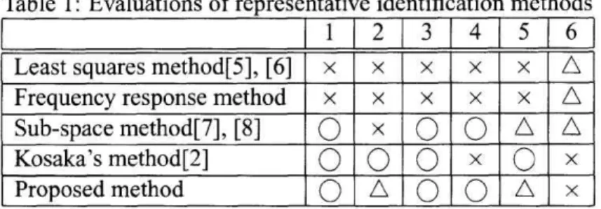
(2) Table 1: Evaluations. of representative. identification. 1. 3. 4. 5. x. x. x. x. 0. Frequency. x. x. x. x. x. 0. 0 0 0. x. 0 0 0. 0. A. A. x. 0. x. 0. A. x. response. method. method. sampling period required in using an M series signal. A conventional least squares method employing a step response restricts the order of an identified model [5]. In the case of servo system, it is desirable that the modelling error is small in low frequency range [4], but least squares methods have a tendency to reduce the error in high frequency range [6]. Sub-space based methods [7, 8] need to obtain a sufficiently large size of, for example, Hankel matrix before deriving its reduced order model, and also use a least squares method in obtaining some system parameters. The method [2] zeroing the 0 N-tuple integral values of output error of single-input singleoutput model has the properties 1, 2, 3, 5 but derives transfer function model.. In this paper, we propose a deterministic off-line identification method [1] that obtains a state-space model by using input and output data with steady state values. The method is composed of the methoc [2] zeroing the 0 N-tuple integral values of outpul error of single-input single-output transfer function model and Ho-Kalman's method [3]. The methoc has an assumptionthat plant system matrix A satisfies ~A < 1 because the method utilizes the Taylor series We prove that the method. car. 0 A. 2.1. Plant. feature. emphasized. is that the derived in low frequency. The paper. is organized. state-space. x (t) = Ax (t) + Bu (t) y (t) = C (t) + Du (t). as follows.. are made. for a plant,. tion method. is stated.. In section. the identified. model. tiveness. are stated.. are illustrated. of the proposed. (1). where t is time and x(t) E RnA, y(t) E RnYand u(t) E Rnu are the state, input and output vector, respectively. 2.2. Assumptions. We make the following assumptions. Al: det (A) A2:. for the system:. 0. C and A satisfy. where det (A) denotes the determinant of A and ay is the integer that satisfies nA+1<a. y<nA+2. ny. (3). model. is. In section. 2. 2.3. oi. The number of acquired input and output data with steady state is nu where those data are denoted as. ny—. range.. assumptions. ical simulations. to be identified. The plant to be identified is represented by the following linear continuous-time nu-input nu-output state-space system:. be applied to plants without the assumption 1A1< 1 The. 6. x. Proposed. of the plant.. 2. Least squares method[5], [6] Sub-space method[7], [8] Kosaka's method[2]. expansion. methods. Identification. algorithm. and the identifica3, the properties. In section. 4, numer-. to indicate. the effec-. method.. ui (t) and yi(t) (i = 1, 2, • • • , nu), respectively, and ui (t)'s satisfy det qui (00) u2 (oo) ... unu (oo)]). 0- (4). From input and output data, U(t) and po(t) are defined as. 2. Identification. algorithm. In this section, assumptions are made for a plant, ant the identification algorithm [1] is stated..

(3) The integer an and np are defined so as to satisfy n<au. < n. nunu. np=. ay+au—. 2.4. + 1 ,(7). Another. identification. algorithm. Another algorithm to identify A by using C0 instead of 0 is stated here.. 1(8). A2' is assumed instead of A2.. where n means the order of the system matrix A in the model. po is derived as. Po = Po(x) •(9). A2':A and B satisfies. pi's (i = 1, 2, • • • , np) are derived as the following equations: _4. where. au is the integer. n. that satisfies. dn. A. Instead of (3), (20), (21) and (22), we respectively use. By using the singular value decomposition, H is decomposed as H. =. By using through. UEVT(17). this algorithm,. the same results. the same procedure. are derived. as the next section.. where E is the diagonal matrix of which elements are. the singular values of H. (ayny x n) matrix 0 and (n x aunu) matrix Co are defined as 3. Properties. In this section,. ,,. of the model. it is shown that the model. corresponds. where MATLABnotation[8] is used. According to with the plant if n = nA without assumption IAl< 1. this notation, A(ai : a2, b1 : b2) means the matrix of As U(t) has steady state from (4) and (5), by uswhich elements the b1. are those in the a1 N a2 columns. and. The estimated system parameter (A, B, C, D) is obtained. ing the final value theorem,. it follows. that. b2 rows in A. by the following. calculations:. det(lirn U(t)) = t—oc. det. limsU( s—o. s)). 0 (32). where s is a complexvariableand x(s) means the Laplacetransformationof x(t). Therefore,using a matrix Ua(s) (det (U,(0)) 0) of whichelements arerationalfunctionsof s, U(s) can be expressedas. where t denotes pseudo inverse matrix..

(4) From (5), (32) and (33), we obtain. where. 6 denotes. yielded. as m.. -. 1. ,.,. 1,_.,1. if). \J. By using the final-value —. a differential. theorem,. we obtain. • • 1 /nl. and then pi+i is yield ed as. P1 is obtained. in the same way as. =. m,(. _. —CA `B.. )(111. •••)(34). Assume that pi(t) (i > 1) satisfies. operator.. pi+i(t) is.

(5) From (25), (35), (47), (48) and (49), we obtain. 0). vliL.,•. Therefore, (37) and (38) follow in ductively. stituting (38) for (16), we get. By sub-. u—. From the above, the model corresponds with the plant. Next we consider that the mothod emphasizes low frequencies. By using the Taylor series expansion around s = 0, the plant (1) is expressed as. If n = nA, from (3), (7), (8), (17), (18), (19), Al , A2 and [3], it follows that. The coefficientsin (51) are derived from low to high order (0 np) in turn, from which A, B, C and D are obtained.. That is, the coefficeients. higher. than n,. are ignored. This leads to emphasize low frequencies because low order coefficients represent the characteristics. in low frequency. range.. From (20), (21) and (43), we get Od =. O„,A-'.. (45). From (45), the pseudo inverse matrix Odt is defined ae. From. Al. 4. Numerical. simulations. In this section, the proposed method is applied to identify 2-input and 2-output system by using step responses of the system. The model is compared with conventional sub-space method [8].. , A2, (22) and (46), we derive 4.1. System. and. simulation. setting. The plant to be identified is as follows:. From Al. , (7), (23), (44) and (47), we obtain. The order of this system nA = 5 and max jAf > 1. ;48). The simulator. is set up as follows:. Sampling. From (3), (24), (43) and (47), we derive. time: 0.01. Data length Input. 49) —31—. signal. step signal. :. 60[s] for. identification. : the. following.

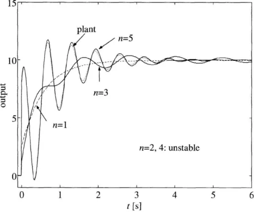
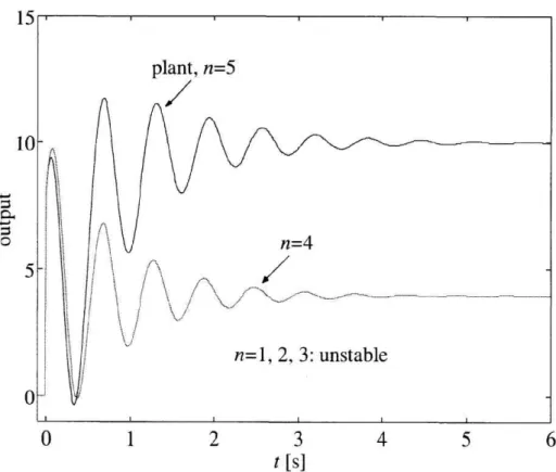
(6) ul (t) _ 212(t) =. (s (t) 0)T (0 s (t) )T. (53). is used. for identification.. The step response. of this. (1 x 1) element of the model is shown in Fig. 2. From Fig. 2, the model. is not good even if n = nA. When. where s(t) is a step function. M series input is used, the models become stable with In the case of the sub-spacemethod, both step sig- Ti= 4, 5. The step responses of these (1 x 1) element nal (54) and M series signal (55) are used for identi- of the models are shown in Fig. 3. From Fig. 3, the fication sub-space method does not emphasize low frequen-. u (t) _(s. (0 (t) 0)T,0 < t <60[s](54) s (t))T, 60 < t < 120[s] u (t) = (ml (t) m2(t))T , 0 < t < 120[455). cies.. wherem(t) is a M series functionwith amplitude1 5. Conclusion. and the minimumperiod 11 samples. The assumption. 4.2. Results. The plant is identified for each n(= 1, 2, • - • , 5). The model stable. identified with. n =. by the proposed 1, 3, 5.. The. method. becomes. step responses. of the. (1 x 1) elements of these models are shown in Fig. 1. From Fig. 1, the proposed method emphasizes low frequencies. In the case of the sub-space method, the model becomes stable only with n = 5 when step input. Figure. 1:. as plant. system. matrix. A satisfies. ~A < 1 of the deterministic off-line state-space model identification method [1] has been taken off. The method can obtain the model from input and output data with constant steady state. It has been verified by numerical simulations that the proposed method emphasizes low frequencies. This method is suitable to identify mechanical systems without genarating noise or vibration because the method can identify MIMO system by using step responce.. Step responses (proposed meth.).

(7) t [sJ Figure. 2:. Step responses (sub-space meth. with step input). 15. Figure. 3:. Step responses (sub-space meth. with M series input).

(8) References [1] M. Kosaka, H. Uda, E. Bamba and H. Shibata: State-spacemodel identificationusing input and output data with steady state values, Proc. of 6th InternationalConference on MechatronicsTechnology(ICMT 2002), pp. 150/155(2002) [2] M. Kosaka, K. Koizumi and H. Shibata: An identification method for a reduced model with zeroing 0 N N-tuple integral values of output error, T. SICE, 36-4, pp. 319/327 (2000) [3] H. P.Zeiger and A. J. McEwen: Approximate linear realization of given dimension via Ho's algorithm, IEEE trans. on Automatic Control, AC-19-2, p. 153, (1974) [4] Z. Zang, R. R. Bitmead and M. Gevers: Iterative weighted least-squares identificationand weighted LQG control design,Automatica, 31-11, pp. 1577/1594,(1995) [5] T. Soderstrom and P. Stoica: System Identification,Prentice-Hall, (1989) [6] B. Wahlberg and L. Ljung: Design variables for bias distribution in transfer function estimation, IEEE trans. on Automatic Control, 31-2, pp. 134/144, (1986) [7] P. Van Overschee and B. De Moor: Subspace identification for linear systems, Kluwer Academic, (1996) [8] L. Ljung: System IdentificationToolbox, The MathWorks, Inc., (1997).

(9)